Product: Abaqus/Standard
This benchmark problem is part of the standard suite of problems designed for Testing Electromagnetic Analysis Methods (TEAM). The problem to be addressed is that of a conducting spherical shell immersed in a time-harmonic uniform magnetic field. The objective is to compute the eddy currents induced in the spherical shell by the magnetic field that is varying in time. Lorentz force and Joule heating in the conductor are also of interest.
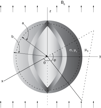
The problem setup is shown in Figure 1.8.51. It depicts a conducting spherical shell immersed in a time-harmonic uniform magnetic field. For visual clarity, the figure depicts a spherical shell with a section of it removed. The inner and outer radius of the conducting spherical shell are ![]() m and
m and ![]() m. Its conductivity and relative magnetic permeability are assumed to be
m. Its conductivity and relative magnetic permeability are assumed to be ![]() S/m and
S/m and ![]() . The magnetic flux density is assumed to have a magnitude of
. The magnetic flux density is assumed to have a magnitude of ![]() T and is oscillating with a frequency of
T and is oscillating with a frequency of ![]() Hz. Without loss of generality, we can assume that the magnetic field is oriented along the
Hz. Without loss of generality, we can assume that the magnetic field is oriented along the ![]() -direction. We will assume that the medium in which the spherical shell is immersed has properties similar to that of a vacuum. For these parameters, the skin depth of the conductor is about
-direction. We will assume that the medium in which the spherical shell is immersed has properties similar to that of a vacuum. For these parameters, the skin depth of the conductor is about ![]() mm, which is smaller than the shell thickness of
mm, which is smaller than the shell thickness of ![]() mm.
mm.
The magnetic vector potential formulation is used to solve this problem. Due to the symmetry of the problem, it is sufficient to model the first octant of the problem domain. Appropriate boundary conditions are imposed on the symmetry planes ![]() ,
, ![]() , and
, and ![]() . Since the magnetic flux density is oriented along the
. Since the magnetic flux density is oriented along the ![]() -direction, azimuthal symmetry of the geometry requires that the total magnetic vector potential
-direction, azimuthal symmetry of the geometry requires that the total magnetic vector potential ![]() is nonzero only in the azimuthal direction. As a result, the magnetic vector potential on the planes
is nonzero only in the azimuthal direction. As a result, the magnetic vector potential on the planes ![]() and
and ![]() is perpendicular to each of these planes. Hence, a homogeneous Dirichlet boundary condition
is perpendicular to each of these planes. Hence, a homogeneous Dirichlet boundary condition ![]() is imposed on the symmetry planes
is imposed on the symmetry planes ![]() and
and ![]() . Symmetry of the problem also requires that the total magnetic field
. Symmetry of the problem also requires that the total magnetic field ![]() on the symmetry plane
on the symmetry plane ![]() be perpendicular to this plane. Hence, a homogeneous Neumann boundary condition
be perpendicular to this plane. Hence, a homogeneous Neumann boundary condition ![]() is applied on the symmetry plane
is applied on the symmetry plane ![]() .
.
Since the problem domain is unbounded, it must be truncated in some way. Abaqus does not support absorbing boundary conditions; therefore, the truncation boundary should be chosen far away from the conductor. Boundary truncation surfaces are chosen such that they are parallel to one of the ![]() ,
, ![]() , or
, or ![]() planes. To demonstrate various boundary conditions that can be applied in an Abaqus/Standard analysis, a spherical boundary surface of radius
planes. To demonstrate various boundary conditions that can be applied in an Abaqus/Standard analysis, a spherical boundary surface of radius ![]() is chosen to truncate the problem domain. Magnetic vector potential and magnetic flux density far away from the conductor are given by
is chosen to truncate the problem domain. Magnetic vector potential and magnetic flux density far away from the conductor are given by ![]() and
and ![]() , where
, where ![]() and
and ![]() are the unit vectors along the
are the unit vectors along the ![]() -coordinate axis and along the azimuthal direction. Clearly neither the projection of magnetic vector potential nor that of magnetic field onto this surface is constant. They vary nonuniformly over the boundary surface. In this problem a nonuniform Dirichlet boundary condition is applied on the spherical boundary surface by supplying a user subroutine UDEMPOTENTIAL that computes the magnetic vector potential on the boundary surface.
-coordinate axis and along the azimuthal direction. Clearly neither the projection of magnetic vector potential nor that of magnetic field onto this surface is constant. They vary nonuniformly over the boundary surface. In this problem a nonuniform Dirichlet boundary condition is applied on the spherical boundary surface by supplying a user subroutine UDEMPOTENTIAL that computes the magnetic vector potential on the boundary surface.
The total magnetic vector potential in various regions can be expressed as follows:
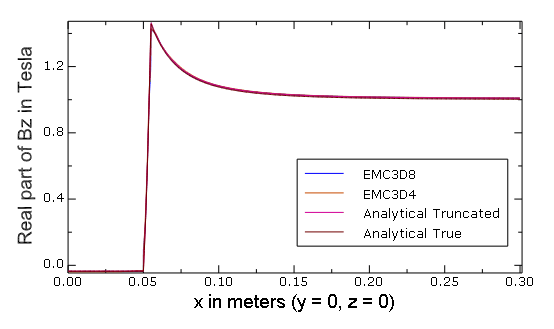
Figure 1.8.52 shows the comparison of the amplitude of the ![]() -component of the magnetic flux density computed using Abaqus/Standard analysis with that of the analytical solution. The labels `EMC3D8' and `EMC3D4' in the legend correspond to the analyses performed with these elements. The labels `Analytical Truncated' and `Analytical True' in the legend correspond to the analytical solution computed by assuming that a Dirichlet boundary condition is applied on an outer spherical boundary surface at a finite distance and at infinity, respectively, as described in the previous section. The figure clearly indicates that the analysis results compare very well with the analytical results and that the outer boundary surface is far enough from the spherical shell that the error introduced by truncation is small.
-component of the magnetic flux density computed using Abaqus/Standard analysis with that of the analytical solution. The labels `EMC3D8' and `EMC3D4' in the legend correspond to the analyses performed with these elements. The labels `Analytical Truncated' and `Analytical True' in the legend correspond to the analytical solution computed by assuming that a Dirichlet boundary condition is applied on an outer spherical boundary surface at a finite distance and at infinity, respectively, as described in the previous section. The figure clearly indicates that the analysis results compare very well with the analytical results and that the outer boundary surface is far enough from the spherical shell that the error introduced by truncation is small.
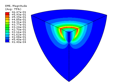
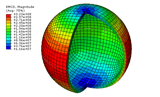
Figure 1.8.53 shows the contour plot of the amplitude of the electric field. Only the first octant of the problem domain is shown in the figure. The view is oriented such that the origin is closer to the reader. For a time-harmonic analysis the amplitude of the electric field is the same as that of the amplitude of the magnetic vector potential scaled by the radian frequency. Finally, Figure 1.8.54 depicts the induced current density in the conductor due to the magnetic field. In the figure a portion of the spherical shell is removed to expose the interior of the shell. The figure shows that the current density in the conductor is larger along the x–y plane and decreases toward the poles. Consequently, the Joule heat generated in the conductor is maximum along the x–y plane.
Eddy current analysis of a conducting spherical shell immersed in a time-harmonic uniform magnetic field using element type EMC3D8, symmetry boundary conditions, and user subroutine UDEMPOTENTIAL.
Eddy current analysis of a conducting spherical shell immersed in a time-harmonic uniform magnetic field using element type EMC3D4, symmetry boundary conditions, and user subroutine UDEMPOTENTIAL.
Emson, C. R. I., “Results for a Hollow Sphere in Uniform Field (Benchmark Problem 6),” The International Journal for Computation and Mathematics in Electrical and Electronic Engineering, vol. 7, pp. 89101, 1988.