Product: Abaqus/Standard
In this example we calculate the acoustic near field scattered from an elastic spherical shell when impinged by a plane wave. The example illustrates the use of simple absorbing boundary conditions, acoustic continuum elements, acoustic infinite elements, tie constraints, and incident wave interactions. The results are compared with a classical solution.
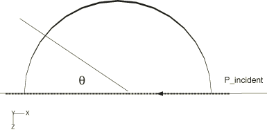
A thin spherical shell of radius ![]() = 0.1 m and thickness h = 0.001 m in an unbounded acoustic medium is subjected to an incident plane wave. The analytical solution for the acoustic scattered pressure is of the form
= 0.1 m and thickness h = 0.001 m in an unbounded acoustic medium is subjected to an incident plane wave. The analytical solution for the acoustic scattered pressure is of the form
![]()
![]()
![]()
![]()
![]()
The finite element mesh uses AC3D20 elements to model the fluid, with an outer radius of ![]() = 0.25 m and a circumferential angle of 10°. Since the problem is axisymmetric, this is sufficient to resolve the field. The shell is meshed with S8R elements, and this mesh is coupled to the acoustic mesh using a tie constraint. Planar incident wave loads of unit reference magnitude are applied to the inner acoustic and outer shell surfaces using *INCIDENT WAVE INTERACTION, REAL, with the standoff point defined at the center of the sphere and the source point defined at a point along the positive x-axis. Specifying the load in this way means that Abaqus will apply loads on the surface corresponding to an incident pressure field having a value of 1 + 0 × i at the standoff point. Two Abaqus models are created: in one, a spherical nonreflecting condition is imposed on the outer surface using the *SIMPEDANCE option; in the other, acoustic infinite elements are created and coupled to the acoustic finite elements using a tie constraint. The material properties used in this problem are shown in Table 1.11.122. The analysis is run using the *STEADY STATE DYNAMICS, DIRECT procedure in the range from 1500 to 5000 Hertz.
= 0.25 m and a circumferential angle of 10°. Since the problem is axisymmetric, this is sufficient to resolve the field. The shell is meshed with S8R elements, and this mesh is coupled to the acoustic mesh using a tie constraint. Planar incident wave loads of unit reference magnitude are applied to the inner acoustic and outer shell surfaces using *INCIDENT WAVE INTERACTION, REAL, with the standoff point defined at the center of the sphere and the source point defined at a point along the positive x-axis. Specifying the load in this way means that Abaqus will apply loads on the surface corresponding to an incident pressure field having a value of 1 + 0 × i at the standoff point. Two Abaqus models are created: in one, a spherical nonreflecting condition is imposed on the outer surface using the *SIMPEDANCE option; in the other, acoustic infinite elements are created and coupled to the acoustic finite elements using a tie constraint. The material properties used in this problem are shown in Table 1.11.122. The analysis is run using the *STEADY STATE DYNAMICS, DIRECT procedure in the range from 1500 to 5000 Hertz.
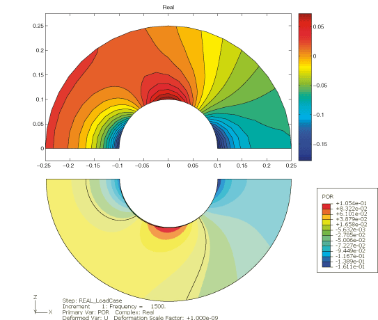
The finite element results for the scattered pressure in the near field, at a frequency of 1500 Hz, are shown in Figure 1.11.122, where they are compared with the analytical values. The figure depicts the analytic near field on the upper annulus and the finite element solution on the lower one. The real parts of the solutions show very good agreement. The analytic solution was not plotted using Abaqus/CAE and has a slightly different color scale.
Model that uses AC3D20 elements and acoustic infinite elements.
Model that uses AC3D20 elements with the Bayliss et al. boundary condition.
Bayliss, A., M. Gunzberger, and E. Turkel, “Boundary Conditions for the Numerical Solution of Elliptic Equations in Exterior Regions,” SIAM Journal of Applied Mathematics, vol. 42, no.2, pp. 430451, 1982.
Junger, M., and D. Feit, Sound, Structures, and Their Interaction, The MIT Press, 1972.
Table 1.11.121 Variable definitions.
| Variable | Definition |
|---|---|
| Scattered acoustic pressure | |
| Elastic contribution to scattered pressure | |
| Rigid contribution to scattered pressure | |
| Incident plane wave coefficient | |
| Legendre polynomial | |
| Spherical Bessel functions of the first kind | |
| Spherical Hankel functions of the first kind | |
| Acoustic wave number | |
| Speed of sound | |
| Frequency | |
| nth resonant frequency of shell in-vacuo, first branch | |
| nth resonant frequency of shell in-vacuo, second branch | |
| Thin-shell section parameter, | |
| Plate wave speed, |