Product: Abaqus/Explicit
This example problem illustrates the following Abaqus features and techniques:
using the Johnson-Holmquist-Beissel (JHB) and the Johnson-Holmquist (JH-2) ceramic material models to study the high-velocity impact of a silicon carbide target. The JHB and JH-2 models are available in Abaqus/Explicit as built-in user materials;
achieving a similar material response for ceramics with proper calibration of the Drucker-Prager plasticity and the equation of state functionality in Abaqus/Explicit; and
comparing numerical results with published results.
Ceramic materials are commonly used in armor protection applications. In recent years Johnson, Holmquist, and their coworkers have developed a series of constitutive relations to simulate the response of ceramic materials under large strain, high-strain rate, and high-pressure impacting conditions. In this example the JHB and JH-2 material models are explored to investigate the penetration velocity of a gold projectile impacting on a silicon carbide target. The computed results are compared with published results given by Holmquist and Johnson (2005).
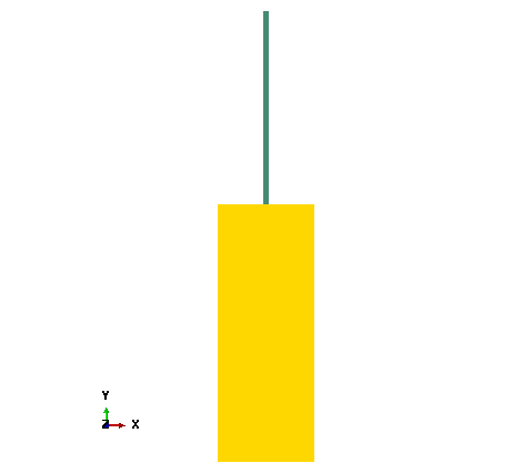
The initial configuration is shown in Figure 2.1.181. Both target and projectile are of cylindrical shape. The silicon carbide target has a radius of 7.5 mm and a length of 40 mm. The gold projectile has a radius of 0.375 mm and a length of 30 mm.
The target material is silicon carbide. This material is very hard and mainly used under compressive load conditions and can only sustain very little tension. Typical applications include bulletproof vests and car brakes due to its high endurance. The strength has a dependence on pressure. In high-speed impact applications, damage to the material plays an important role in the evolution of the strength. The totally failed silicon carbide will not sustain any load. The projectile is gold, which is soft compared to the target material.
Three cases are investigated, each using a different approach to model the silicon carbide material: the first case uses the JHB material model, the second uses the JH-2 model, and the third case uses a combination of several Abaqus options to obtain a similar constitutive model within a more general framework. The Lagrangian description is used for both projectile and target. General contact with surface erosion is used for all three cases. Element deletion and node erosion are considered. A tonne-millimeter-second unit system was chosen for all simulations.
| Case 1 | JHB (built-in user material) |
| Case 2 | JH-2 (built-in user material) |
| Case 3 | Combination of Drucker-Prager plasticity, equation of state, and Johnson-Cook rate dependence |
The sections that follow discuss the analysis considerations that are applicable to all cases.
An Abaqus/Explicit dynamic analysis is used for all the simulations. The total duration for the penetration process is 7 μs.
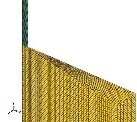
An 11.5° slice of the cylinders is modeled. There are five elements along the radial direction of the projectile. The element size along the radial direction for the target is nearly the same as for the projectile. Due to the large radius ratio between the projectile and the target, there are 343,980 elements for the target and 2000 elements for the projectile. Figure 2.1.182 shows part of the meshes used for the analysis.
The different material models used for the silicon carbide target are discussed in detail in subsequent sections. The JHB and JH-2 models are available as built-in user materials for Abaqus (i.e., via VUMAT subroutines that are built-in). These built-in materials are invoked by using material names starting with ABQ_JHB and ABQ_JH2, respectively. For descriptions of the ceramic material models, see “Analyzing ceramics with the Johnson-Holmquist and Johnson-Holmquist-Beissel material models” in the Dassault Systèmes DSX.ECO Knowledge Base at www.3ds.com/support/knowledge-base or the SIMULIA Online Support System, which is accessible through the My Support page at www.simulia.com.
The material for the projectile is gold. The density is 19,240 kg/m3. The shear modulus is 27.2 GPa. The hydrodynamic behavior is described by the Mie-Grüneisen equation of state. The linear ![]() Hugoniot form is used. The parameters are
Hugoniot form is used. The parameters are ![]() = 2946.16 m/s,
= 2946.16 m/s, ![]() = 3.08623, and
= 3.08623, and ![]() = 2.8. The strength is 130 MPa described as a perfect plasticity. A ductile damage initiation criterion with the equivalent plastic strain of 0.2 at the onset of damage is used. The fracture energy is chosen as 0 for the damage evolution.
= 2.8. The strength is 130 MPa described as a perfect plasticity. A ductile damage initiation criterion with the equivalent plastic strain of 0.2 at the onset of damage is used. The fracture energy is chosen as 0 for the damage evolution.
Initial velocity conditions of 4000 m/s are specified for all the nodes of the projectile in the axial direction toward the target.
All the nodes on the symmetry axis, which is set up as the global x-direction, can move only along this axis, so zero velocity boundary conditions are prescribed for both the y- and z-directions. To satisfy the axial symmetry boundary conditions, a cylindrical coordinate system is established. The circumferential degrees of freedom for all the nodes on the two side surfaces except the nodes on the symmetry axis of both the target and the projectile are prescribed with zero velocity boundary conditions. The nodes on the non-impacting end of the target are fixed along the axial direction.
General contact is used to model the interactions between the projectile and the target. The interior surface of both the target and the projectile is included to enable element removal.
There is only one explicit dynamic analysis step, during which the penetration takes place.
In addition to the standard output identifiers available in Abaqus, the solution-dependent state variables described in Table 2.1.181 and Table 2.1.182 are also available for output for the JHB and JH-2 models, respectively.
This section provides a detailed description of the different constitutive models for ceramic materials that are used to model the silicon carbide target for each of the cases considered.
This case uses the JHB model for the silicon carbide target. The JHB material parameters for silicon carbide given in Holmquist and Johnson (2005) are used in this study. They are listed in Table 2.1.183.
The JHB model consists of three main components: a representation of the deviatoric strength of the intact and fractured material in the form of a pressure-dependent yield surface, a damage model that transitions the material from the intact state to a fractured state, and an equation of state (EOS) for the pressure-density relation that can include dilation (or bulking) effects as well as a phase change (not considered in this study).
The strength of the material is expressed in terms of the von Mises equivalent stress, ![]() , and is a function of the pressure,
, and is a function of the pressure, ![]() , the dimensionless equivalent strain rate,
, the dimensionless equivalent strain rate, ![]() (where
(where ![]() is the equivalent plastic strain rate and
is the equivalent plastic strain rate and ![]() is the reference strain rate), and the damage variable,
is the reference strain rate), and the damage variable, ![]() (
(![]() ). For the intact (undamaged) material,
). For the intact (undamaged) material, ![]() , whereas
, whereas ![]() for a fully damaged material.
for a fully damaged material.
For a dimensionless strain rate of ![]() , the strength of the intact material (
, the strength of the intact material (![]() ) takes the form
) takes the form
![]()
![]()
![]()
![]()
The intact and fractured strengths above are for a dimensionless strain rate of ![]() . The effect from strain rates is incorporated by the Johnson-Cook strain rate dependence law as
. The effect from strain rates is incorporated by the Johnson-Cook strain rate dependence law as ![]() , where
, where ![]() is the strength corresponding to
is the strength corresponding to ![]() . Plastic flow is volume preserving and is governed by a Mises flow potential.
. Plastic flow is volume preserving and is governed by a Mises flow potential.
The damage initiation parameter, ![]() , accumulates with plastic strain according to
, accumulates with plastic strain according to
![]()
![]()
The JHB model assumes that the material fails immediately, ![]() when
when ![]() . For other values of
. For other values of ![]() , there is no damage (
, there is no damage (![]() ) and the material preserves its intact strength.
) and the material preserves its intact strength.
The equations for the pressure-density relationship without phase change are used in this study and are listed here.
![]()
![]()
![]()
![]()
The second case uses the JH-2 model. Unlike the JHB model, the JH-2 model assumes that the damage variable increases progressively with plastic deformation. The material parameters used for the JH-2 model are listed in Table 2.1.184. The JH-2 model similarly consists of three components.
The strength of the material is expressed in terms of the normalized von Mises equivalent stress as
![]()
![]()
![]()
The damage initiation parameter, ![]() , accumulates with plastic strain according to
, accumulates with plastic strain according to
![]()
![]()
The equations for the pressure-density relationship are similar to the JHB model.
![]()
![]()
![]()
![]()
We use a combination of the Drucker-Prager plasticity model and an equation of state to obtain a material behavior that is similar to that of the JH-2 model. In this way, we are not confined to follow the specific expressions and subsequently the material parameters of the JH models. So we can take advantage of the generality of the Drucker-Prager plasticity model and the different equations of state available in Abaqus. To conform to the above JH material models, we also cast the description with three components for the Drucker-Prager plasticity model.
We use the general exponent form of the extended Drucker-Prager model (“Extended Drucker-Prager models,” Section 22.3.1 of the Abaqus Analysis User's Manual) which, after some manipulations, can be written in the following form:
![]()
![]()
![]()
![]()
![]()
![]()
The ductile damage initiation criterion in Abaqus (“Damage initiation for ductile metals,” Section 23.2.2 of the Abaqus Analysis User's Manual) can be calibrated to reproduce the damage criterion used in the JH-2 damage model. The ductile criterion requires the specification of the equivalent plastic strain at the onset of damage as a function of the stress triaxiality. Along the intact strength curve of the JH-2 model, the stress triaxiality is given as
![]()
![]()
![]()
The Mie-Grüneisen equation of state (“Mie-Grüneisen equations of state” in “Equation of state,” Section 24.2.1 of the Abaqus Analysis User's Manual) is used to describe the hydrodynamic behavior of the silicon carbide material. The linear ![]() Hugoniot form is used. Without the energy contribution (
Hugoniot form is used. Without the energy contribution (![]() = 0.0), the pressure is expressed as
= 0.0), the pressure is expressed as
![]()
![]()
![]()
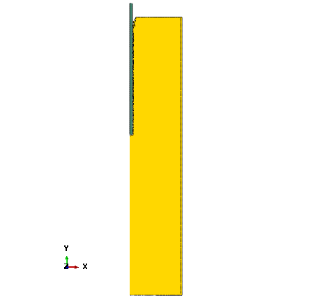
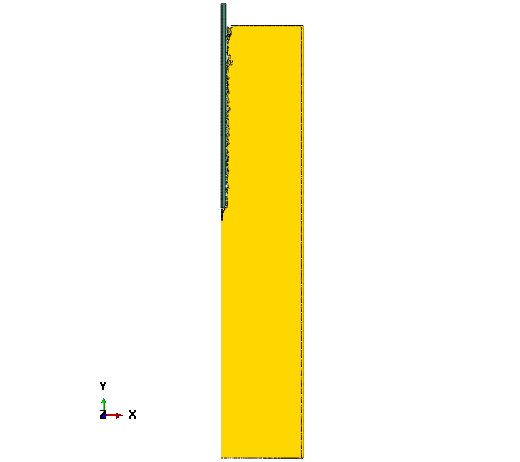
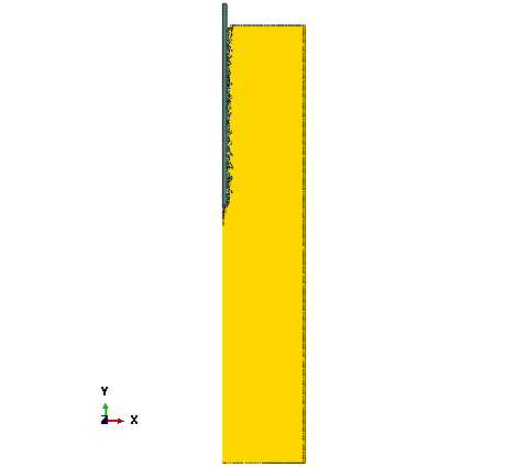
The penetration depths from the three models and the published results in the reference by Holmquist and Johnson (2005) at 3 μs, 5 μs, and 7 μs are listed in Table 2.1.185. All results from the three models match the published results well. Especially, the results obtained with the Drucker-Prager model are in satisfactory agreement with all other results obtained with the JH models. The final configurations for the JHB, JH-2, and Drucker-Prager models are shown in Figure 2.1.183, Figure 2.1.184, and Figure 2.1.185, respectively.
Input file to create and analyze the model.
Input file to create and analyze the model.
Input file to create and analyze the model.
Holmquist, T. J., Johnson, G. R., “Characterization and Evaluation of Silicon Carbide for High-Velocity Impact,” Journal of Applied Physics, vol. 97, 093502, 2005.
Johnson, G. R., Holmquist, T. J., “An Improved Computational Constitutive Model for Brittle Materials,” High Pressure Science and Technology–1993, New York, AIP Press, 1993.
Table 2.1.181 Solution-dependent state variables defined in JHB model.
| Output variables | Symbol | Description |
|---|---|---|
| SDV1 | Equivalent plastic strain PEEQ | |
| SDV2 | Equivalent plastic strain rate | |
| SDV3 | Damage initiation criterion | |
| SDV4 | Damage variable | |
| SDV5 | Pressure increment due to bulking | |
| SDV6 | Yield strength | |
| SDV7 | Maximum value of volumetric strain | |
| SDV8 | Volumetric strain | |
| SDV9 | Material point status: 1 if active, 0 if failed |
Table 2.1.182 Solution-dependent state variables defined in JH-2 model.
| Output variables | Symbol | Description |
|---|---|---|
| SDV1 | Equivalent plastic strain PEEQ | |
| SDV2 | Equivalent plastic strain rate | |
| SDV3 | Damage initiation criterion | |
| SDV4 | Damage variable | |
| SDV5 | Pressure increment due to bulking | |
| SDV6 | Yield strength | |
| SDV7 | Volumetric strain | |
| SDV8 | Material point status: 1 if active, 0 if failed |
Table 2.1.183 Material parameters for JHB model.
| Line 1 | ||||||||
| 3215 kg/m3 | 193 GPa | 4.92 GPa | 1.5 GPa | 0.1 GPa | 0.25 GPa | 0.009 | 1.0 | |
| Line 2 | ||||||||
| 0.75 GPa | 12.2 GPa | 0.2 GPa | 1.0 | |||||
| Line 3 | FS | |||||||
| 0.16 | 1.0 | 999 | 0.2 | |||||
| Line 4 | ||||||||
| 220 GPa | 361 GPa | 0 GPa | ||||||
| Line 5 | ||||||||
| 0 | 0 | 0 | 0 | 0 | 0 | 0 |