Products: Abaqus/Standard Abaqus/CFD Abaqus/CAE
This example demonstrates the following Abaqus features and techniques for Abaqus/CFD to Abaqus/Standard co-simulation:
using Abaqus/CFD to Abaqus/Standard co-simulation to analyze a conjugate heat transfer problem,
solving both the laminar flow field and buoyancy-driven natural convection heat transfer occurring external to a structure in Abaqus/CFD, and
solving for the heat transfer within the structure using Abaqus/Standard.
This example examines the transient conjugate heat transfer between a single printed circuit board (PCB)–mounted electronic component and the ambient air. The component is subjected to a passive power dissipation that results in the transfer of heat both within the component and the PCB due to conduction. Furthermore, the heated surface of the component and the PCB induces a temperature-dependent density differential in the surrounding air, thereby setting up a buoyancy-driven natural convection process external to the surface. Heat is thus transferred from the component and PCB surfaces to the ambient air through this convection process. Understanding the resulting conduction-convection conjugate heat transfer phenomenon results in more accurate damage estimation and life prediction for electronic components.
The details of the model are largely derived from Eveloy and Rodgers (2005).
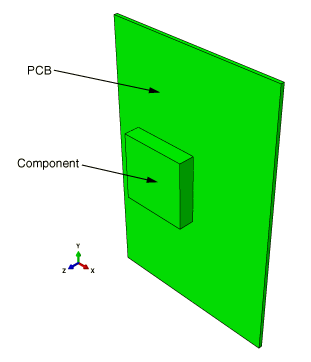
Nominal component/PCB geometry dimensions are considered. The PCB dimensions are 7.8 × 11.6 × 0.16 cm. The mounted electronic component consists of an encapsulant of dimension 3 × 3 × 0.7 cm that encapsulates a heat slug of dimension 1.8 × 1.8 × 0.3 cm mounted atop a die of dimension 0.75 × 0.75 × 0.2 cm. The assembled PCB-component package is shown in Figure 6.1.11. The cross-section view of the assembled package is shown in Figure 6.1.12. The size of the computational domain that encloses the electronic package is taken to be 27.8 × 20 × 12.56 cm for the Abaqus/CFD flow computations.
The PCB material has a thermal conductivity of 19.25 W/m/K, a density of 8950 kg/m3, a specific heat of 1300 J/kg/K, and a thermal expansion of 1.6 × 10⁵ /K. The heat slug material has a thermal conductivity of 398 W/m/K, a density of 8940 kg/m3, a specific heat of 385 J/kg/K, and a thermal expansion of 3.3 × 10⁶ /K. The die material has a thermal conductivity of 130.1 W/m/K, a density of 2330 kg/m3, a specific heat of 712 J/kg/K, and a thermal expansion of 3.3 × 10⁶ /K. The encapsulant material has a thermal conductivity of 0.63 W/m/K, a density of 1820 kg/m3, a specific heat of 882 J/kg/K, and a thermal expansion of 1.9 × 10⁵ /K. For the external fluid domain, properties of air, namely a density of 1.127 kg/m3, a thermal conductivity of 2.71 × 10² W/m/K, a specific heat of 1006.4 J/kg/K, a thermal expansion of 3.43 × 10³ /K, and a viscosity of 1.983 × 10⁵ kg/m/s, are assumed.
The initial temperature of the assembled electronic package and the external fluid (ambient air) is set to 293 K. In addition, the fluid is initially assumed to be quiescent and, hence, its velocity is set to zero everywhere.
The electronic component of the assembled package is subjected to a passive power dissipation corresponding to a specified body heat flux value of 5 × 10⁷ W/m3. The bottom surface of the external computational domain is assumed to be a rigid floor, and an adiabatic wall condition is assumed there. The electronic package is firmly attached to the bottom of the computational domain, as shown in Figure 6.1.13. The computational domain boundaries for the external flow and heat transfer calculations are positioned at sufficient distances from the assembled electronic package such that the effects of the boundaries on the results are negligible. A no-slip, no-penetration flow wall boundary condition is enforced at the bottom surface. At the top, an outlet boundary condition is specified with the fluid pressure set to zero. For all other boundaries, free-stream conditions are applied for both the velocity and temperature.
Gravity loading is applied along the negative y-axis (see Figure 6.1.13).
The component-mounted circuit board is subjected to volumetric power dissipation, which generates heat within the structure. Heat transfer to the surface of the structure takes place via conduction. The heated surface then generates a buoyancy-driven natural convection in the surrounding ambient air.
The Abaqus/CFD to Abaqus/Standard co-simulation approach is used to solve the conjugate heat transfer problem. The Abaqus/Standard model of the co-simulation consists of the component-mounted PCB electronic package (see Figure 6.1.11). The Abaqus/CFD model of the co-simulation consists of the external region bounding the electronic package (see Figure 6.1.13). Co-simulation regions across which data will be exchanged during the co-simulation analysis are identified on each model at the location of the electronic package surface.
The Abaqus/Standard model includes a transient heat transfer step. The Abaqus/CFD model includes an incompressible laminar flow analysis coupled with the energy equation that governs the temperature distribution.
The Abaqus/Standard model is meshed with linear hexahedral (DC3D8) elements. The Abaqus/CFD model is meshed with linear hexahedral (FC3D8) fluid elements.
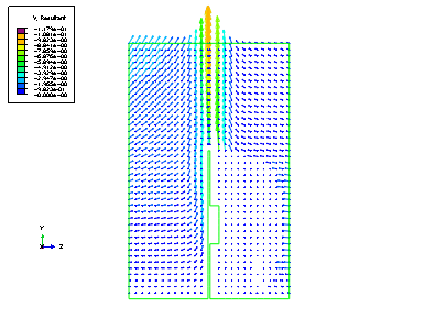
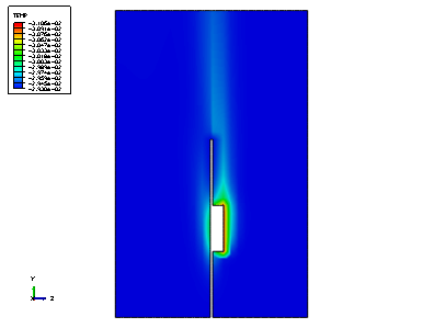
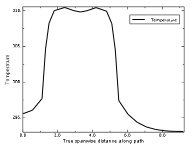
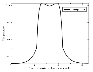
The heat generated within the electronic component gets distributed to its surface and also to the surface of the PCB substrate by conduction. The heated air near the component surface becomes less dense and rises upward due to buoyancy. The Grashof number (a parameter describing the ratio of buoyancy to viscous forces) for this problem, based on the board length, was estimated to be of the order 106 as reported by Eveloy and Rodgers (2005). Because of incompressibility, the upward rising air entrains cold air from the surroundings, thereby setting up a natural convection flow. The upward rising hot air and entrained cold air from the sides are illustrated in Figure 6.1.14, where the velocity vectors (V) are plotted on the center cross-sectional slice of the domain in the y–z plane. In Figure 6.1.14 entrainment from the out-of-plane direction appears as small dots. The contours of temperature distribution (TEMP) on the same cross-sectional slice are shown in Figure 6.1.15, where the hot electronic component surface and the upward rising thermal plume can be clearly seen. The temperature distribution (NT11) along a particular path in the spanwise direction (x-axis) on the surface of the component-mounted electronic package is shown in Figure 6.1.16. Heat is seen to spread from the component surface (the area of near-constant heat distribution) to the surfaces of the PCB substrate on either side. The temperature distribution (NT11) along a particular path in the streamwise direction (y-axis) on the surface of the electronic package shown in Figure 6.1.17 illustrates the same phenomenon. These distributions are qualitatively similar to the experimentally measured temperature profiles given in Eveloy and Rodgers (2005).
Script to generate the model in Abaqus/CAE using the orphan meshes from cfd_mesh.inp and std_heat_transfer.inp.
Orphan mesh for the Abaqus/CFD domain.
Orphan mesh for the Abaqus/Standard domain.
Figure 6.1.12 Cross-sectional view of the electronic package indicating the different materials forming the component and circuit board.
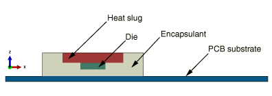
Figure 6.1.13 Electronic package anchored to the bottom of the computational domain (enclosing box).
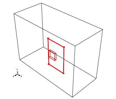
Figure 6.1.14 Plot of velocity vectors induced due to natural convection on a cross-sectional slice.