Product: Abaqus/CAE
Benefits: Abaqus/CAE now offers mapped fields that allow you to define spatially varying parameter values from an external data source. This feature allows the definition of certain properties and attributes from data generated in a third-party CAE application or from an Abaqus output database.
Description: Abaqus/CAE now provides two types of analytical fields: mapped fields and the previously available expression fields. You can create and manage analytical fields using the Analytical Field toolset in the Property module, Interaction module, or Load module.
For example, you can define a spatially varying shell thickness or pressure load by providing the thickness or pressure values at different coordinates. Parameter values can be read in from a point cloud data file generated by a third-party CAE application or from an Abaqus output database (.odb) file.
Mapped fields allow you to import discrete and discontinuous parameter data and apply it to your Abaqus/CAE model. Abaqus/CAE applies the values to the current model, mapping the imported X-, Y-, and Z-coordinates to locations in the model. Abaqus/CAE maps the source data onto the target model, and Abaqus computes the distributed parameter values to be used during the analysis. The parameter values are also called field values, or field data; for example, pressure values at different points on a surface.
Mapped fields can be used to define the attributes and properties shown in Table 41.
Table 41 Attributes and properties that support mapped fields.
| Category | Attribute/Property |
|---|---|
| Loads | Pressure |
| Boundary conditions | Temperature |
| Pore pressure | |
| Acoustic pressure | |
| Mass concentration | |
| Mass flow | |
| Electrical potential | |
| Predefined fields | Nodal temperature |
| Pore pressure | |
| Void ratio | |
| Saturation | |
| Interactions | Surface film condition |
| Surface radiative | |
| Concentrated film condition | |
| Other | Density (material density distributions) |
| Shell thicknesses (element distribution or nodal distribution in shell sections) |
The magnitude you specify in the load, boundary condition, predefined field, or interaction is used as a multiplier for the mapped field data values. Mapped fields can be used only in three-dimensional models.
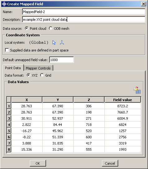
Figure 47 shows the Edit Mapped Field dialog box used to create mapped fields.
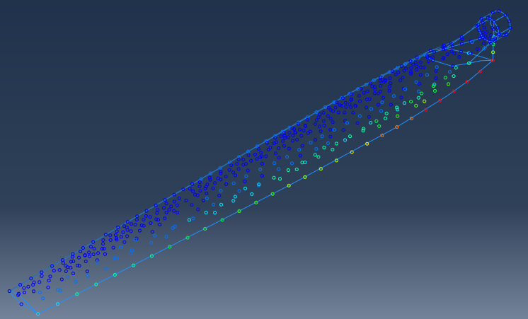
You can display symbols to visualize the locations and relative magnitudes of the source data points for point cloud data in XYZ format, as shown in Figure 48.
When the source data are taken from an output database, the process is called mesh-to-mesh mapping. An example of mesh-to-mesh mapping is demonstrated in the following workflow:
Set up and run a thermal analysis in Abaqus to generate an output database that contains nodal temperatures.
Open the output database in the Visualization module, and display the undeformed contour plot of a specific results step and frame for output variable NT.
Open the model database that contains your main target model, and create a mapped analytical field using the nodal temperature values displayed in the viewport in the previous step as the source data.
Mesh (or remesh) your target model.
Create a temperature predefined field, and select the mapped analytical field to define the temperature distribution. Abaqus/CAE maps the source data points and their associated temperatures onto points in the target model.
Set up and run the subsequent analysis.
Property module, Interaction module, or Load module: ToolsAnalytical Field