
Products: Abaqus/Standard Abaqus/Explicit Abaqus/CAE
The submodeling technique:
is used to study a local part of a model with a refined mesh based on interpolation of the solution from an initial (undeformed), relatively coarse, global model;
is most useful when it is necessary to obtain an accurate, detailed solution in a local region and the detailed modeling of that local region has negligible effect on the overall solution;
can be used to drive a local part of the model by nodal results, such as displacements (see “Node-based submodeling,” later in this section), or by the element stress results (see “Surface-based submodeling,” later in this section) from the global mesh;
can be used to analyze an acoustic model driven by displacements from a structural, global model when the acoustic fluid has negligible effect on the structural solution;
can be used for the analysis of a structure driven by acoustic pressures from an acoustic or coupled acoustic-structural, global model;
can use a combination of Abaqus/Explicit and Abaqus/Standard procedures;
can use a combination of linear and nonlinear procedures; and
cannot be used in an import analysis.
The model whose solution is interpolated onto the relevant parts of the boundary of the submodel is referred to as the “global” model (even though it may itself be a submodel of a larger “global” model). Driven variables are defined as those variables in the submodel that are constrained to match results from the global model. Driven variables can be degrees of freedom at nodes in the node-based technique, or they can be components of stress tensor at the integration points of element faces in the surface-based technique.
Submodeling can be applied quite generally in Abaqus. The material response defined for the submodel may be different from that defined for the global model. Both the global model and the submodel can have nonlinear response. See “Shell-to-solid submodeling and shell-to-solid coupling of a pipe joint,” Section 1.1.10 of the Abaqus Example Problems Manual, for an example application of the submodeling technique.
Submodeling is classified first according to which of two basic techniques is used. The most common, and more general technique, is node-based submodeling, which uses a nodal results field (including displacement, temperature, or pressure degrees of freedom) to interpolate global model results onto the submodel nodes. The alternative surface-based technique uses the stress field to interpolate global model results onto the submodel integration points on the driven element-based surface facets.
You can choose either the node-based or surface-based technique or a combination of the two in your submodel. The following factors should be considered in deciding on the technique to be used:
Whether you are performing solid-to-solid submodeling in a general static analysis in Abaqus/Standard:
Surface-based submodeling is available only for solid models and static analyses.
For all other procedures use the node-based technique.
Whether the global model and submodel differ significantly in their average stiffness in the region of the submodel:
When the stiffness of the models is comparable, node-based submodeling of displacements will provide comparable results to the surface-based technique with a lesser likelihood of numerical issues associated with rigid-body modes.
When the stiffness of the models differs and the global model is exposed primarily to a load-controlled environment, the surface-based technique will generally provide more accurate stress results. Stiffness differences may arise due to additional detail in the submodel, such as explicit modeling of a fillet or a hole. In other cases stiffness changes may result from minor geometry changes for which a reanalysis of the global model is not warranted.
Whether your model is subjected to large deformations or rotations:
Node-based submodeling of displacements will result in more accurate transmission of large deformation and rotation to the submodel.
Whether the displacement response of the global model corresponds to the displacement response of the submodel:
When the displacements in the global model correspond closely with the expected displacements in the submodel, node-based submodeling is generally preferable.
Surface-based submodeling should be used when the submodel displacement response is expected to differ from the global model response. This situation can occur when thermal strains are modeled and the temperature history of the submodel differs from that of the global model; for example, when heat transfer submodeling is performed as part of a sequential thermal-structural analysis.
The stiffness of the structure:
Surface-based submodeling may provide more accurate results for very stiff structures. When the structure is so stiff that only a small component of the global model displacement field contributes to the stress response, numerical roundoff in the displacement results can become significant; for example, when the global model displacement is dominated by a rigid-body motion component.
The type of output you are interested in from the submodel:
Node-based submodeling of displacements will result in more accurate transmission of a displacement field.
Surface-based submodeling will result in more accurate transmission of a stress field, and determination of reaction forces in the submodel.
You can use both node-based submodeling and stress-based submodeling in the same model.
Node-based submodeling is the more general technique, supporting a variety of element type combinations and procedures in both Abaqus/Explicit and Abaqus/Standard.
| Input File Usage: | *SUBMODEL, TYPE=NODE |
| Abaqus/CAE Usage: | Load module: Create Boundary Condition: choose Other for the Category and Submodel for the Types for Selected Step: Driving region: Specify |
Different element types can be used in the submodel than those used to model the corresponding region in the global model.
The following types of submodeling are provided for the node-based approach (global-to-submodel):
Two-dimensional models:
Solid-to-solid
Acoustic-to-structure
Three-dimensional models:
Solid-to-solid
Shell-to-shell
Membrane-to-membrane
Shell-to-solid
Acoustic-to-structure
Both the global model and the submodel can have nonlinear response and can be analyzed for any sequence of analysis procedures. These procedures do not have to be the same for both models. For example, the linear or nonlinear dynamic response of the global model can be used to drive the static, nonlinear response of the submodel on the grounds that the submodel is too small for dynamic effects to be significant in that local region. The global procedure can be performed in Abaqus/Standard to drive a submodeling procedure in Abaqus/Explicit and vice versa. For example, a static analysis performed in Abaqus/Standard can drive a quasi-static Abaqus/Explicit analysis in the submodel. The step time used in these analyses can be different; the time variable of the amplitude functions generated at the driven nodes can be scaled to the step time used in the submodel.
Your submodel cannot refer to a global model step that includes multiple load cases (see “Multiple load case analysis,” Section 6.1.3). You must perform the global analysis with a single load definition for the step that will drive the submodel.
Surface-based submodeling is provided as a complement to the node-based technique, enabling you to drive the submodel with stresses from the global model.
| Input File Usage: | *SUBMODEL, TYPE=SURFACE |
| Abaqus/CAE Usage: | Load module: Create Load: choose Mechanical for the Category and Submodel for the Types for Selected Step: Driving region: Specify |
The following types of submodeling are provided for the surface-based approach (global-to-submodel):
Two-dimensional models:
Solid-to-solid
Three-dimensional models:
Solid-to-solid
Different element types can be used in the submodel than those used to model the corresponding region in the global model. Continuum elements supported for the static analysis procedure are supported for surface-based submodeling, with the following exceptions:
Cylindrical elements are not supported.
Continuum shell elements are not supported.
The surface-based technique is implemented only for static analysis in Abaqus/Standard.
Your submodel cannot refer to a global model step that includes multiple load cases (see “Multiple load case analysis,” Section 6.1.3). You must perform the global analysis with a single load definition for the step that will drive the submodel.
A submodeling analysis consists of:
running a global analysis and saving the results in the vicinity of the submodel boundary;
defining the total set of driven nodes or driven surfaces in the submodel;
defining the time variation of the driven variables in the submodel analysis by specifying the actual nodes and degrees of freedom or element-based surfaces to be driven in each step; and
running the submodel analysis using the “driven variables” to drive the solution.
The submodel is run as a separate analysis from the global analysis. The only link between the submodel and the global model is the transfer of the time-dependent values of variables saved in the global analysis to the relevant boundary nodes of the submodel or to the relevant boundary surfaces. This transfer is accomplished by saving the results from the global model either in the results (.fil) file or in the output database (.odb) for the node-based technique or in the output database (.odb) for the stress-based technique, then reading these results into the submodel analysis. If the global model is defined in terms of an assembly of part instances, the part (.prt) file from the global model is required for the submodel analysis. Since the submodel is a separate analysis, submodeling can be used to any number of levels; a submodel can be used as the global model for a subsequent submodel.
The global model in a submodeling analysis must define the submodel boundary response with sufficient accuracy. It is your responsibility to ensure that any particular use of the submodeling technique provides physically meaningful results. In general, the solution at the boundary of the submodel must not be altered significantly by the different local modeling. There is no built-in check of this criterion in Abaqus; it is a matter of judgment on your part. In general, accuracy can be checked by comparing contour plots of important variables near the boundaries of the submodeled region.
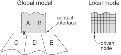
By default, the global model in the vicinity of the submodel is searched for elements that encompass the locations of driven nodes or driven surfaces' faces; the submodel is then driven by the response of these elements. In some cases more than one element can encompass the location of a driven node. For example, adjacent bodies in the global model may have temporarily coincident nodes or surfaces, as depicted in Figure 10.2.11.
Figure 10.2.11 A global model with coincident surfaces in the area of the local model's driven nodes.
To preclude certain elements from driving the submodel, you have the option of specifying a global element set to limit the search to an appropriate subset of the global model.
| Input File Usage: | *SUBMODEL, GLOBAL ELSET=name |
If the global model is defined in terms of an assembly of part instances, give the complete name—including the assembly and part instance names—when specifying the global element set. For example, an element set named top in part instance I-1 of assembly Assembly-1 must be referred to by Assembly-1.I-1.top. If the submodel is not defined in terms of an assembly of part instances, the dots in the global element set name must be replaced by underscores: Assembly-1_I-1_top. If the global element set is defined at the assembly level, you may provide the element set name without qualifying it with the assembly name in a submodel analysis. |
| Abaqus/CAE Usage: | Load module: Create Boundary Condition: choose Other for the Category and Submodel for the Types for Selected Step: Driving region: Specify |
The size of the results file or the output database can be minimized for a submodeling analysis by requesting output for only those global nodes and global elements that are used to drive the submodel. To determine which global nodes and/or elements are used to drive the submodel, do the following:
Run a data check analysis on the global model with any combination of results file or output database file output requests. A data check analysis is performed by using the datacheck parameter in the command for running Abaqus (“Abaqus/Standard, Abaqus/Explicit, and Abaqus/CFD execution,” Section 3.2.2).
Run a data check analysis on the submodel.
Pay special attention to the frequency at which you request output in the global model (see “Output to the data and results files,” Section 4.1.2, and “Output to the output database,” Section 4.1.3). It is possible to define the results file output or nodal and element output to the output database file such that the information is written at different frequencies for different nodes and elements, although that should not be done for nodes and elements involved in the interpolation to define values at driven variables since Abaqus will take values at the coarsest frequency only. To avoid this problem, write the nodal and elemental output to the output database or the results file using the same frequency for all nodes and elements involved in the interpolation and choose a frequency that will allow the history in the submodel to be reproduced accurately.
| Input File Usage: | To control the output frequency to the Abaqus/Standard results file, use the following option: |
*NODE FILE, FREQUENCY To control the output frequency to the Abaqus/Explicit results file, use the following option: *FILE OUTPUT, NUMBER INTERVAL To control the output frequency to the output database, use the following option: *OUTPUT, FIELD, FREQUENCY |
| Abaqus/CAE Usage: | Step module: Output |
Any of the material models described in Part V, “Materials,” can be used in the global and submodel analyses. The material response defined for the submodel may be different from that defined for the global model.
The dimensionality of the submodel must be the same as that of the global model: both models must be either two-dimensional or three-dimensional. The following limitations apply:
The boundary nodes of the submodel must lie within regions of the global model where Abaqus is able to perform spatial interpolation to define the values of the driven variables. Therefore, they must lie within (or, as allowed by the exterior tolerance, near to) two- or three-dimensional geometrically defined elements in the global model. Such geometrically defined elements are:
first- or second-order triangles or quadrilaterals in two dimensions;
first- or second-order triangular or quadrilateral shells; and
first- or second-order tetrahedra, wedges, or bricks in three dimensions.
The boundary nodes cannot lie in regions of the global model where there are only one-dimensional elements (beams, trusses, links, axisymmetric shells) since Abaqus does not provide the necessary interpolation of results for such elements.
The boundary nodes cannot lie in regions of the global model where there are only user elements, substructures, springs, dashpots, cohesive elements, etc. since those element types do not allow for geometric interpolation.
The boundary nodes cannot lie in regions of the global model where there are only axisymmetric solid elements with nonlinear, asymmetric deformation (CAXA elements). The submodeling capability is currently not supported for these elements.
The reference node associated with generalized plane strain elements (CPEG) cannot be used as a driven boundary node in a submodeling analysis.
Any of the output normally available within a particular procedure is also available during a submodeling analysis (see “Abaqus/Standard output variable identifiers,” Section 4.2.1, and “Abaqus/Explicit output variable identifiers,” Section 4.2.2).
As described above, nodal output requests to the results file or output database file must be used in the global analysis to save the values of the driven variables at the submodel boundary.