Products: Abaqus/Standard Abaqus/CAE
“Defining general contact interactions in Abaqus/Standard,” Section 34.2.1
“Defining general contact,” Section 15.13.1 of the Abaqus/CAE User's Manual
“Defining surface-to-surface contact,” Section 15.13.6 of the Abaqus/CAE User's Manual
“Defining self-contact,” Section 15.13.7 of the Abaqus/CAE User's Manual
“Using contact and constraint detection,” Section 15.16 of the Abaqus/CAE User's Manual
Abaqus/Standard provides several contact fomulations. Each formulation is based on a choice of a contact discretization, a tracking approach, and assignment of “master” and “slave” roles to the contact surfaces. For general contact interactions, the discretization, tracking approach, and surface role assignments are selected automatically by Abaqus/Standard; for contact pairs, you can specify these aspects of the contact formulation using the interface described in “Defining contact pairs in Abaqus/Standard,” Section 34.3.1. The default contact formulation is applicable in most situations, but you may find it desirable to choose another formulation in some cases. This section discusses in detail the formulations that Abaqus/Standard uses in contact simulations.
Your choice of a tracking approach will have a considerable impact on how contact surfaces interact. In Abaqus/Standard there are two tracking approaches to account for the relative motion of two interacting surfaces in mechanical contact simulations:
finite sliding, which is the most general and allows any arbitrary motion of the surfaces (see “Finite-sliding interaction between deformable bodies,” Section 5.1.2 of the Abaqus Theory Manual, and “Finite-sliding interaction between a deformable and a rigid body,” Section 5.1.3 of the Abaqus Theory Manual); and
small sliding, which assumes that although two bodies may undergo large motions, there will be relatively little sliding of one surface along the other (see “Small-sliding interaction between bodies,” Section 5.1.1 of the Abaqus Theory Manual).
General contact in Abaqus/Standard always uses the finite-sliding, surface-to-surface contact formulation. This formulation can also be used for contact pairs, but it is not the default. The discussions in this section of finite-sliding, surface-to-surface contact apply equally to general contact and to contact pairs.
In a general contact domain the master and slave roles are assigned to surfaces automatically, although it is possible to override these default assignments. The behavior of master surfaces and slave surfaces is consistent across general contact and contact pair interactions. The specification of master and slave surfaces in a general contact domain is covered in detail in “Numerical controls for general contact in Abaqus/Standard,” Section 34.2.6.
Abaqus/Standard applies conditional constraints at various locations on interacting surfaces to simulate contact conditions. The locations and conditions of these constraints depend on the contact discretization used in the overall contact formulation. Abaqus/Standard offers two contact discretization options: a traditional “node-to-surface” discretization and a true “surface-to-surface” discretization.
With traditional node-to-surface discretization the contact conditions are established such that each “slave” node on one side of a contact interface effectively interacts with a point of projection on the “master” surface on the opposite side of the contact interface (see Figure 36.1.11). Thus, each contact condition involves a single slave node and a group of nearby master nodes from which values are interpolated to the projection point.
Traditional node-to-surface discretization has the following characteristics:
The slave nodes are constrained not to penetrate into the master surface; however, the nodes of the master surface can, in principle, penetrate into the slave surface (for example, see the case on the upper-right of Figure 36.1.12).
The contact direction is based on the normal of the master surface.
The only information needed for the slave surface is the location and surface area associated with each node; the direction of the slave surface normal and slave surface curvature are not relevant. Thus, the slave surface can be defined as a group of nodes—a node-based surface.
Node-to-surface discretization is available even if a node-based surface is not used in a contact pair definition.
Surface-to-surface discretization considers the shape of both the slave and master surfaces in the region of contact constraints. Surface-to-surface discretization has the following key characteristics:
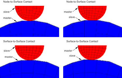
The surface-to-surface formulation enforces contact conditions in an average sense over regions nearby slave nodes rather than only at individual slave nodes. The averaging regions are approximately centered on slave nodes, so each contact constraint will predominantly consider one slave node but will also consider adjacent slave nodes. Some penetration may be observed at individual nodes; however, large, undetected penetrations of master nodes into the slave surface do not occur with this discretization. Figure 36.1.12 compares contact enforcement for node-to-surface and surface-to-surface contact for an example with dissimilar mesh refinement on the contacting bodies.
The contact direction is based on an average normal of the slave surface in the region surrounding a slave node.
Surface-to-surface discretization is not applicable if a node-based surface is used in the contact pair definition.
In general, surface-to-surface discretization provides more accurate stress and pressure results than node-to-surface discretization if the surface geometry is reasonably well represented by the contact surfaces. Figure 36.1.13 shows an example of improved contact pressure accuracy with surface-to-surface contact compared to node-to-surface contact.
Figure 36.1.13 Comparison of contact pressure accuracy for node-to-surface and surface-to-surface contact discretizations.
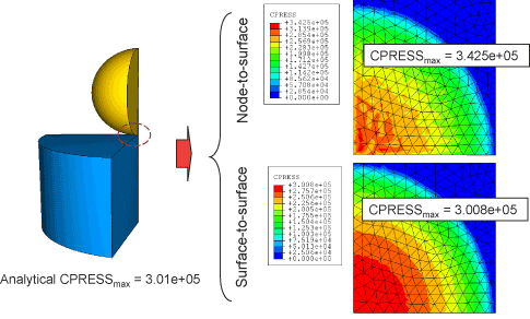
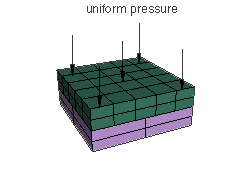
Contact using surface-to-surface discretization is also less sensitive to master and slave surface designations than node-to-surface contact (see “Choosing the master and slave roles in a two-surface contact pair” below). Figure 36.1.14 shows a simple model involving two blocks with dissimilar mesh densities.
The bottom block is fixed to the ground, and a uniform pressure of 100 Pa is applied to the top face of the top block. Analytically, the top block should exert a uniform pressure of 100 Pa on the bottom block across the entire contact interface. Table 36.1.11 compares the Abaqus analysis results for different contact discretizations and slave surface designations.Table 36.1.11 Error (from analytical results) for various discretization/slave surface combinations.
| Contact discretization | Slave Surface | Maximum error in CPRESS |
|---|---|---|
| Node-to-surface | Top block | 13% |
| Bottom block | 31% | |
| Surface-to-surface | Top block | ~1% |
| Bottom block | ~1% |
If the surface geometry is not well-represented due to the use of a coarse mesh, significant inaccuracies can exist regardless of whether surface-to-surface contact or node-to-surface contact is used. In some cases surface smoothing techniques available for surface-to-surface contact can significantly improve solutions obtained with a coarse mesh. See “Smoothing contact surfaces in Abaqus/Standard,” Section 36.1.3, for a discussion of surface smoothing options for surface-to-surface contact.
Surface-to-surface discretization generally involves more nodes per constraint and can, therefore, increase solution cost. In most applications the extra cost is fairly small, but the cost can become significant in some cases. The following factors (especially in combination) can lead to surface-to-surface contact being costly:
A large fraction of the model is involved in contact.
The master surface is more refined than the slave surface.
Multiple layers of shells are involved in contact, such that the master surface of one contact pair acts as the slave surface of another contact pair.
The surface-to-surface formulation is primarily intended for common situations in which normal directions of contacting surfaces are approximately opposite. The node-to-surface contact formulation is often preferable for treating contact involving feature edges or corners if the respective slave and master facet normal directions are not approximately opposite in the active contact region.
In Abaqus/Standard there are two tracking approaches to account for the relative motion of two interacting surfaces in mechanical contact simulations.
Finite-sliding contact is the most general tracking approach and allows for arbitrary relative separation, sliding, and rotation of the contacting surfaces. For finite-sliding contact the connectivity of the currently active contact constraints changes upon relative tangential motion of the contacting surfaces. For a detailed description of how Abaqus/Standard calculates finite-sliding contact, see “Using the finite-sliding tracking approach” later in this section.
Small-sliding contact assumes that there will be relatively little sliding of one surface along the other and is based on linearized approximations of the master surface per constraint. The groups of nodes involved with individual contact constraints are fixed throughout the analysis for small-sliding contact, although the active/inactive status of these constraints typically can change during the analysis. You should consider using small-sliding contact when the approximations are reasonable, due to computational savings and added robustness. For a detailed description of how Abaqus/Standard calculates small-sliding contact, see “Using the small-sliding tracking approach” later in this section.
Abaqus/Standard enforces the following rules related to the assignment of the master and slave roles for contact surfaces:
Analytical rigid surfaces and rigid-element-based surfaces must always be the master surface.
A node-based surface can act only as a slave surface and always uses node-to-surface contact.
Slave surfaces must always be attached to deformable bodies or deformable bodies defined as rigid.
Both surfaces in a contact pair cannot be rigid surfaces with the exception of deformable surfaces defined as rigid (see “Rigid body definition,” Section 2.4.1).
When both surfaces in a contact pair are element-based and attached to either deformable bodies or deformable bodies defined as rigid, you have to choose which surface will be the slave surface and which will be the master surface. This choice is particularly important for node-to-surface contact. Generally, if a smaller surface contacts a larger surface, it is best to choose the smaller surface as the slave surface. If that distinction cannot be made, the master surface should be chosen as the surface of the stiffer body or as the surface with the coarser mesh if the two surfaces are on structures with comparable stiffnesses. The stiffness of the structure and not just the material should be considered when choosing the master and slave surface. For example, a thin sheet of metal may be less stiff than a larger block of rubber even though the steel has a larger modulus than the rubber material. If the stiffness and mesh density are the same on both surfaces, the preferred choice is not always obvious.
The choice of master and slave roles typically has much less effect on the results with a surface-to-surface contact formulation than with a node-to-surface contact formulation. However, the assignment of master and slave roles can have a significant effect on performance with surface-to-surface contact if the two surfaces have dissimilar mesh refinement; the solution can become quite expensive if the slave surface is much coarser than the master surface.
Your choice of contact discretization and tracking approach have considerable impact on an analysis. In addition to the qualities already discussed, certain combinations of discretizations and tracking approaches have their own characteristics and limitations associated with them. These characteristics are summarized in Table 36.1.12. You should also consider the solution costs associated with the various contact formulations.
Table 36.1.12 Comparison of contact formulation characteristics.
| Characteristic | Contact formulation | |||
|---|---|---|---|---|
| Node-to-surface | Surface-to-surface | |||
| Finite-sliding | Small-sliding | Finite-sliding | Small-sliding | |
| Account for shell thickness by default | No | Yes | Yes | Yes |
| Allow self-contact | Yes | No | Yes | No |
| Allow double-sided surfaces | Slave surface only | Slave surface only | Yes1 | Yes |
| Surface smoothing by default | Some smoothing of master surface | Yes for anchor points; each constraint uses flat approximation of master surface | No | No for anchor points; each constraint uses flat approximation of master surface |
| Default constraint enforcement method | Augmented Lagrange method for 3-D self-contact; otherwise, direct method | Direct method | Penalty method | Direct method |
| Ensure moment equilibrium for offset reference surfaces with friction | No | No | Yes | Yes |
| 1Double-sided master surfaces are allowed with the finite-sliding, surface-to-surface formulation only if the path-based tracking algorithm is used (see “Path-based versus state-based tracking algorithms”). Double-sided slave surfaces are allowed with both tracking algorithms if the master surface is not user defined. | ||||
Most contact formulations will account for the surface thickness of a shell when calculating contact constraints. However, the finite-sliding, node-to-surface formulation will not account for shell thicknesses. These calculations are discussed in more detail in “Accounting for shell and membrane thickness” in “Assigning surface properties for contact pairs in Abaqus/Standard,” Section 34.3.2.
Self-contact is typically the result of large deformation in a model. It is often difficult to predict which regions will be involved in the contact or how they will move relative to each other. Therefore, self-contact cannot use the small-sliding tracking approach.
Doubled-sided contact surfaces based on shell-like elements are allowed to act as slave and/or master surfaces for the surface-to-surface contact formulation by default and are allowed to act as the slave surface for the node-to-surface contact formulation. For a shell-like surface to act as the master surface for the surface-to-surface formulation with the optional state-based tracking algorithm (see “Path-based versus state-based tracking algorithms” below) or for the node-to-surface contact formulation, the surface must be defined as single-sided (see “Defining single-sided surfaces” in “Element-based surface definition,” Section 2.3.2, and “Orientation considerations for shell-like surfaces” in “Defining contact pairs in Abaqus/Standard,” Section 34.3.1, for more information).
When using node-to-surface discretization, corners or small protrusions of a jagged master surface are allowed to penetrate the spaces between nodes in the node-based surface. It is sometimes possible for a slave node sliding along the master surface to snag on these corners. Therefore, Abaqus/Standard automatically smooths the master surface for contact calculations utilizing node-to-surface discretization to minimize this phenomenon. The details are discussed further in “Smoothing master surfaces for the finite-sliding, node-to-surface formulation” later in this section.
No surface smoothing occurs by default when using surface-to-surface discretization. Surface-to-surface discretization considers contact conditions in an average sense over a finite region, which tends to alleviate problems associated with small protrusions of the master surface penetrating the slave surface and introduces some inherent smoothing characteristics at the constraint level. However, this inherent smoothing typically does not significantly mitigate errors associated with poor geometric representations of curved surfaces when a relatively coarse mesh is used. In some cases nondefault circumferential or spherical surface smoothing methods available for surface-to-surface contact can significantly improve solutions obtained with a coarse mesh (see “Smoothing contact surfaces in Abaqus/Standard,” Section 36.1.3).
In many cases Abaqus/Standard strictly enforces the contact constraints discussed previously by default. However, strict enforcement of contact constraints can sometimes lead to overconstraint issues (for example, see “Overconstraint checks,” Section 33.6.1) or convergence difficulty. To address these issues and allow for decreased solution cost with typically minimal sacrifice to solution accuracy, Abaqus/Standard also provides penalty-based constraint enforcement methods. The numerical constraint enforcement methods (and defaults) are discussed in detail in “Contact constraint enforcement methods in Abaqus/Standard,” Section 36.1.2.
Based on Newton's third law of motion, contact forces should be self-equilibrating; that is, the net contact forces acting on the respective surfaces for each active contact constraint should be equal and opposite and effectively act through a common point. Contact constraints based on surface-to-surface contact discretization always exhibit this characteristic. Contact constraints based on node-to-surface discretization always generate zero net force, but under certain circumstances can generate a net moment in the numerical solution. Frictional forces associated with node-to-surface contact constraints will generate net moment if an offset exists between the respective reference surfaces. The following factors can contribute to a normal-direction offset between nodes of respective contact surfaces while contact constraints are active:
The presence of a softened pressure-versus-overclosure behavior (due to a user-specified, softened pressure-overclosure model or use of a constraint enforcement method, such as the penalty method, that exhibits numerical softening.
Contact calculations accounting for shell or membrane thicknesses (which is not allowed with the finite-sliding, node-to-surface formulation).
User-specified initial contact clearances (see “Defining a precise initial clearance or overclosure for small-sliding contact” in “Adjusting initial surface positions and specifying initial clearances in Abaqus/Standard contact pairs,” Section 34.3.5).
Various usages of special-purpose contact elements, such as tube-to-tube contact elements (see “Contact modeling with elements,” Section 38.1.1, and “Tube-to-tube contact elements,” Section 38.3.1), result in some normal distance between nodes that interact with each other.
There is no easy way to predict which contact discretization method will result in lower overall solution cost. Basic trends include:
Node-to-surface contact discretization tends to be less costly per iteration than surface-to-surface contact discretization (because surface-to-surface contact discretization generally involves more nodes per constraint).
Contact conditions with finite-sliding contact tend to converge in fewer iterations with surface-to-surface contact discretization than with node-to-surface contact discretization (because surface-to-surface contact discretization has more continuous behavior upon sliding).
The finite-sliding tracking approach allows for arbitrary separation, sliding, and rotation of the surfaces. Abaqus/Standard contact pairs use a finite-sliding, node-to-surface contact formulation by default. General contact in Abaqus/Standard always uses a finite-sliding, surface-to-surface contact formulation.
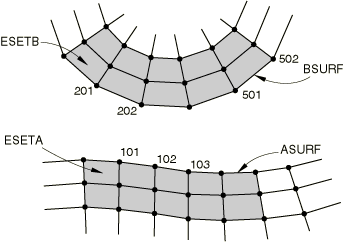
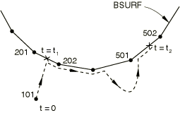
Consider the case shown in Figure 36.1.15, with surface ASURF acting as the slave surface to surface BSURF in a finite-sliding, node-to-surface contact pair.
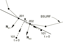
In this example slave node 101 may come into contact anywhere along the master surface BSURF. While in contact, it is constrained to slide along BSURF, irrespective of the orientation and deformation of this surface. This behavior is possible because Abaqus/Standard tracks the position of node 101 relative to the master surface BSURF as the bodies deform. Figure 36.1.16 shows the possible evolution of the contact between node 101 and its master surface BSURF.
Node 101 is in contact with the element face with end nodes 201 and 202 at timeBrief descriptions of the tracking algorithms available in Abaqus/Standard are provided below so that you can be aware of their characteristics and available options.
The “path-based” tracking algorithm carefully considers the relative paths of points on the slave surface with respect to the master surface within each increment and allows for double-sided shell and membrane master surfaces. The path-based tracking algorithm is available only for finite-sliding, surface-to-surface contact interactions involving element-based master surfaces and is the default for those interactions. The path-based algorithm is sometimes more effective than the state-based algorithm for analyses involving self-contact or large incremental relative motion.
| Input File Usage: | Use the following option to specify use of the path-based tracking algorithm: |
*CONTACT PAIR, INTERACTION=interaction_property_name, TYPE=SURFACE TO SURFACE, TRACKING=PATH |
| Abaqus/CAE Usage: | Interaction module: surface-to-surface contact or self-contact interaction editor: Discretization method: Surface to surface, Contact tracking: Two configurations (path) |
The “state-based” tracking algorithm updates the tracking state based on the tracking state associated with the beginning of the increment together with geometric information associated with the predicted configuration. This algorithm is well-suited for most finite-sliding analyses but requires the use of single-sided surfaces and occasionally has difficulty tracking large incremental motion. State-based tracking may miss detecting contact if the incremental relative motion exceeds the dimensions of the master surface or if the incremental motion cuts across corners of the master surface; specifying an upper bound for the increment size helps avoid these problems. The state-based tracking algorithm is:
the only tracking algorithm available for finite-sliding, node-to-surface contact pairs;
the only tracking algorithm available for finite-sliding contact interactions involving an analytical rigid master surface;
a non-default option for finite-sliding, surface-to-surface contact pairs involving an element-based master surface.
| Input File Usage: | Use the following option to specify use of the state-based tracking algorithm: |
*CONTACT PAIR, INTERACTION=interaction_property_name, TYPE=SURFACE TO SURFACE, TRACKING=STATE |
| Abaqus/CAE Usage: | Interaction module: surface-to-surface contact or self-contact interaction editor: Discretization method: Surface to surface, Contact tracking: Single configuration (state) |
The finite-sliding, node-to-surface contact formulation requires that master surfaces have continuous surface normals at all points. Convergence problems can result if master surfaces that do not have continuous surface normals are used in finite-sliding, node-to-surface contact analyses; slave nodes tend to get “stuck” at points where the master surface normals are discontinuous. Abaqus/Standard automatically smooths the surface normals of element-based master surfaces (see “Smoothing deformable master surfaces and rigid surfaces defined with rigid elements” below) used in finite-sliding, node-to-surface contact simulations, including those modeled with slide lines. You are expected to create smooth analytical rigid surfaces (see “Analytical rigid surface definition,” Section 2.3.4). No such smoothing of master surface normals is needed with the finite-sliding, surface-to-surface formulation.
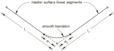
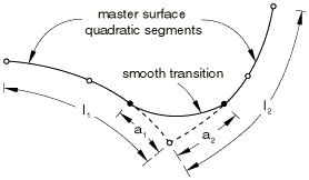
For finite-sliding, node-to-surface contact simulations with planar or axisymmetric deformable master surfaces, Abaqus/Standard will smooth any discontinuous transitions between two first-order element faces with parabolic curves. Discontinuous transitions between two second-order element faces are smoothed with cubic curves connecting two points located on the element's faces. This smoothing is shown in Figure 36.1.17 for first-order elements (linear segments) and in Figure 36.1.18 for second-order elements (parabolic segments). For finite-sliding, node-to-surface simulations with three-dimensional deformable master surfaces and rigid master surfaces using rigid elements, Abaqus/Standard will smooth any discontinuous surface normal transitions between the master surface facets.
You can control the degree of smoothing of the master surface in node-to-surface contact simulations or in analyses using slide lines and contact elements by specifying a fraction f. The default value of f is 0.2.
For planar or axisymmetric deformable master surfaces, ![]() , where
, where ![]() and
and ![]() are the lengths of the element facets that join at the surface node and
are the lengths of the element facets that join at the surface node and ![]() (see Figure 36.1.17 and Figure 36.1.18). Abaqus/Standard will construct either a parabolic or a cubic segment between two points at distances
(see Figure 36.1.17 and Figure 36.1.18). Abaqus/Standard will construct either a parabolic or a cubic segment between two points at distances ![]() and
and ![]() from the node at which the discontinuity exists; this smoothed segment will be used in the contact calculations. Thus, the contact surface will differ from the faceted element geometry. Smoothing affects only segments where the normal to the deformable master surface is discontinuous at the node joining two elements: it does not affect the two segments adjacent to the midside nodes on second-order element faces.
from the node at which the discontinuity exists; this smoothed segment will be used in the contact calculations. Thus, the contact surface will differ from the faceted element geometry. Smoothing affects only segments where the normal to the deformable master surface is discontinuous at the node joining two elements: it does not affect the two segments adjacent to the midside nodes on second-order element faces.
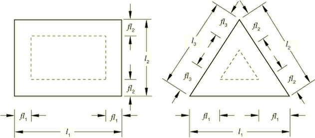
For three-dimensional, element-based master surfaces, f is defined as a fraction of the dimension of a facet as shown in Figure 36.1.19. The normal vector of a point within the region bounded by the dashed lines is computed to be normal to the facet. Outside this region the normal is smoothed with respect to the adjacent facets, using a generalization of the two-dimensional approach shown in Figure 36.1.17 and Figure 36.1.18. The physical geometry of a three-dimensional facet is not smoothed; only the surface normal definitions associated with the facet are affected by the smoothing operation. The implementation of the normal-direction smoothing algorithm is slightly different for surfaces based on rigid type elements (see “Rigid elements,” Section 29.3.1) than other element types. This difference typically has minimal effect on the convergence behavior or solution results; however, for example, different solution behavior may occasionally be observed between otherwise identical analyses in which a rigid body is modeled with R3D4 elements in one case and S4R elements assigned to a rigid body in another case.
| Input File Usage: | Use the following option for node-to-surface contact simulations: |
*CONTACT PAIR, INTERACTION=interaction_property_name, SMOOTH=f Use the following option when using slide lines and contact elements: *SLIDE LINE, ELSET=name, SMOOTH=f |
| Abaqus/CAE Usage: | Interaction module: Interaction |
When a two-dimensional or axisymmetric deformable master surface ends at a symmetry plane and node-to-surface discretization is used, Abaqus/Standard will smooth and calculate the proper surface normals and tangent planes of the end segment if the boundary condition at the symmetry end is specified with the symmetry “type” boundary XSYMM or YSYMM. This smoothing procedure is accomplished by reflecting the end segment about the symmetry plane and constructing either a parabolic or a cubic segment between the end segment and the reflected segment. Thus, the contact surface may differ from the faceted element geometry near the end. Abaqus/Standard will automatically adjust the surface normal and tangent planes at ![]() of an axisymmetric master surface regardless of whether a symmetry boundary condition is defined. The small- and finite-sliding, surface-to-surface formulations have no special treatment for master surfaces ending at a symmetry plane. See “Modifying the master surface normals” in “Contact formulations in Abaqus/Standard,” Section 36.1.1, for a discussion of how the small-sliding, node-to-surface formulation treats master surfaces ending at a symmetry plane.
of an axisymmetric master surface regardless of whether a symmetry boundary condition is defined. The small- and finite-sliding, surface-to-surface formulations have no special treatment for master surfaces ending at a symmetry plane. See “Modifying the master surface normals” in “Contact formulations in Abaqus/Standard,” Section 36.1.1, for a discussion of how the small-sliding, node-to-surface formulation treats master surfaces ending at a symmetry plane.
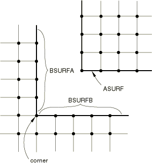
To model a master surface with corners in two dimensions (fold lines in three dimensions), break the surface into multiple surfaces. This technique prevents Abaqus/Standard from smoothing out the corners or fold lines and allows Abaqus/Standard to introduce constraints associated with each surface if a slave node is in contact with an interior corner or fold in the master surface.
To accurately model the master surface with a corner shown in Figure 36.1.110, you must define two contact pairs: the first contact pair has ASURF as the slave surface and BSURFA as the master surface; the second contact pair has ASURF as the slave surface and BSURFB as the master surface.
Finite-sliding simulations usually include nonlinear geometric effects because such simulations generally involve large deformations and large rotations. However, it is also possible to use the finite-sliding tracking approach in a geometrically linear analysis (see “Geometric nonlinearity” in “General and linear perturbation procedures,” Section 6.1.2). The load transfer paths between the surfaces and the contact direction are updated in finite-sliding, geometrically linear analyses. This capability is useful for analyzing finite sliding between two stiff bodies that do not undergo large rotations.
Normal contact constraints due to node-to-surface discretization produce unsymmetric terms in the system of equations when three-dimensional faceted surfaces come in contact. These terms have a strong effect on the convergence rate in regions on the master surfaces with large differences in surface normals between facets.
Normal contact constraints due to surface-to-surface discretization produce unsymmetric terms in both two- and three-dimensional cases. These terms have a strong effect on the convergence rate in regions where the master and slave surfaces are not parallel to each other.
In both cases you should use the unsymmetric solution scheme for the step to improve the convergence rate of the simulation (see “Matrix storage and solution scheme in Abaqus/Standard” in “Procedures: overview,” Section 6.1.1).
Contact simulations that involve strong frictional effects can also produce unsymmetric terms. See “Unsymmetric terms in the system of equations” in “Frictional behavior,” Section 35.1.5, for details.
For a large class of contact problems the general tracking of the finite-sliding approach is unnecessary, even though geometric nonlinearity may need to be considered. Abaqus/Standard provides a small-sliding tracking approach for such problems. For geometrically nonlinear analyses this formulation assumes that the surfaces may undergo arbitrarily large rotations but that a slave node will interact with the same local area of the master surface throughout the analysis. For geometrically linear analyses the small-sliding approach reduces to an infinitesimal-sliding and rotation approach, in which it is assumed that both the relative motion of the surfaces and the absolute motion of the contacting bodies are small.
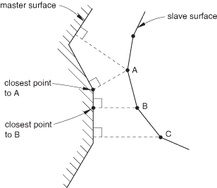
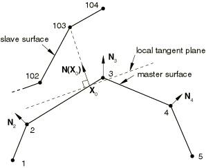
Abaqus/Standard attempts to associate a planar approximation of the master surface with each slave node of a small-sliding contact pair. Contact interactions are considered between a given slave node (or region nearby a given slave node for the surface-to-surface formulation) and the associated local tangent plane. An example for the small-sliding, node-to-surface formulation is shown in Figure 36.1.111 (for example, the slave node is typically constrained not to penetrate this local tangent plane). Each local tangent plane, which is a line in two dimensions, is defined by an anchor point, ![]() , on the master surface and an orientation vector at the anchor point (see Figure 36.1.111).
, on the master surface and an orientation vector at the anchor point (see Figure 36.1.111).
Figure 36.1.111 Definition of the anchor point and local tangent plane used by the small-sliding, node-to-surface formulation for node 103.
Having a local tangent plane for each slave node means that for the small-sliding tracking approach Abaqus/Standard does not have to monitor slave nodes for possible contact along the entire master surface. Therefore, small-sliding contact is generally less expensive computationally than finite-sliding contact. The cost savings are often most dramatic in three-dimensional contact problems.
For node-to-surface contact Abaqus/Standard chooses the anchor point of a slave node's local tangent plane such that the vector from the anchor point to the slave node coincides with a smoothly varying normal vector on the master surface. The anchor point is chosen before the analysis starts using the initial configuration of the model.
The algorithm requires that the master surface have a smoothly varying normal vector ![]() , where
, where ![]() is any point on the master surface. The first step in defining
is any point on the master surface. The first step in defining ![]() is to construct the unit normal vectors at each node of the master surface. Abaqus/Standard forms these nodal normals by averaging the normals of the element faces making up the master surface; only the element faces in the surface definition will contribute to the nodal normals and, thus, to
is to construct the unit normal vectors at each node of the master surface. Abaqus/Standard forms these nodal normals by averaging the normals of the element faces making up the master surface; only the element faces in the surface definition will contribute to the nodal normals and, thus, to ![]() . Abaqus/Standard uses the initial nodal coordinates to compute these normals.
. Abaqus/Standard uses the initial nodal coordinates to compute these normals.
Figure 36.1.111 shows the nodal unit normals for a master surface, the anchor point ![]() , and the local tangent plane associated with slave node 103. Abaqus/Standard uses the nodal unit normals
, and the local tangent plane associated with slave node 103. Abaqus/Standard uses the nodal unit normals ![]() and
and ![]() , along with the shape functions of the element containing the two nodes, to construct
, along with the shape functions of the element containing the two nodes, to construct ![]() on the 2–3 element face. Abaqus/Standard chooses the anchor point
on the 2–3 element face. Abaqus/Standard chooses the anchor point ![]() of the local tangent plane for node 103 so that
of the local tangent plane for node 103 so that ![]() passes through node 103.
passes through node 103. ![]() is the contact direction for slave node 103 and defines the orientation of the local tangent plane. In this example, as in many cases, the local tangent plane is only an approximation of the actual mesh geometry.
is the contact direction for slave node 103 and defines the orientation of the local tangent plane. In this example, as in many cases, the local tangent plane is only an approximation of the actual mesh geometry.
Sometimes the default smoothed master surface normal and the local tangent plane that Abaqus/Standard calculates are not suitable for the desired analysis. The most common situation where unsuitable surface normals are calculated occurs when a curved master surface ends at a symmetry plane and the boundary conditions have been specified in direct format rather than in symmetry “type” format (XSYMM, YSYMM, or ZSYMM—see “Boundary conditions in Abaqus/Standard and Abaqus/Explicit,” Section 32.3.1). In this case the correct normals should be in the symmetry plane; however, because the surface facets that abut the symmetry plane usually form an angle with the plane, the normal will project away from the symmetry plane. The effect of this behavior can be that a slave node does not have a normal from the master surface pass through it (the slave node is said not to “intersect” the master surface). No contact constraints will be enforced for such slave nodes.
A message is printed in the data (.dat) file whenever a slave node does not intersect its master surface. By specifying the proper symmetry “type” boundary condition, Abaqus/Standard will calculate the correct normal and local tangent planes along the symmetry planes of the master surface.
If the smoothed normals of the master surface and the local tangent planes calculated by Abaqus/Standard are unsuitable and it is not feasible to apply symmetry “type” boundary conditions, several other methods are available for modifying the smoothed normals. One method is to add or remove some of the element faces making up the master surface. However, this method can influence only the surface normals near the perimeter of the master surface.
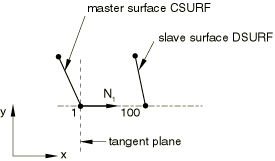
The other method is to modify the nodal normals on the master surface by defining user-specified normals (see “Normal definitions at nodes,” Section 2.1.4). This method is especially useful in providing a more accurate representation of the surface geometry. Figure 36.1.112 shows two concentric cylinders that contact each other; the inner cylinder is chosen as the master surface CSURF.
Figure 36.1.112 Master surface normal at node 1 in a small-sliding model of concentric cylinders. With the default ![]() slave node 100 will never contact CSURF.
slave node 100 will never contact CSURF.
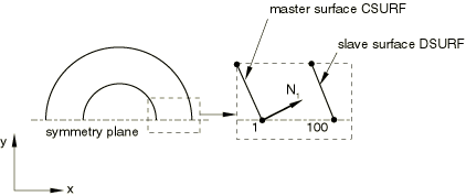
If a half-symmetry model is used, the default master surface normal at the symmetry plane will cause problems. As shown in Figure 36.1.112, the nodal normal ![]() does not point along the symmetry plane, which means that slave node 100 will never intersect the master surface. In a small-sliding problem if a slave node fails to intersect the master surface at the start of the analysis, it will be free to penetrate the master surface because no local tangent plane will be formed. Abaqus/Standard provides the initial contact status—open, overclosed, or “no intersection”—in the data file for every slave node in the model (see “Contact diagnostics in an Abaqus/Standard analysis,” Section 37.1.1). Use this information to confirm that the necessary tangent planes for a model have been found.
does not point along the symmetry plane, which means that slave node 100 will never intersect the master surface. In a small-sliding problem if a slave node fails to intersect the master surface at the start of the analysis, it will be free to penetrate the master surface because no local tangent plane will be formed. Abaqus/Standard provides the initial contact status—open, overclosed, or “no intersection”—in the data file for every slave node in the model (see “Contact diagnostics in an Abaqus/Standard analysis,” Section 37.1.1). Use this information to confirm that the necessary tangent planes for a model have been found.
In situations such as that shown in Figure 36.1.112, define a YSYMM “type” boundary condition at node 1 to specify the symmetry plane. The master normal at the node on the symmetry plane will be modified to lie along the symmetry plane, allowing slave node 100 to see the master surface CSURF. The small- and finite-sliding, surface-to-surface formulations have no special treatment for master surfaces ending at a symmetry plane. See “Smoothing a deformable master surface along symmetry edges” in “Contact formulations in Abaqus/Standard,” Section 36.1.1, for a discussion of how the finite-sliding, node-to-surface formulation treats master surfaces ending at a symmetry plane.
In situations where a symmetry “type” boundary condition cannot be specified, define a user-specified normal (1.00E+00, 0.00E+00, 0.00E+00) at node 1 on the master surface CSURF to correct the problem. This method will also allow slave node 100 to see the master surface.
The modification to CSURF's normal at node 1, which makes CSURF a better approximation of the actual surface, is shown in Figure 36.1.113.
A key difference with the surface-to-surface approach is that more than one slave node is involved in each contact constraint—this is related to the fact that the surface-to-surface formulation enforces contact conditions in an average sense over regions nearby slave nodes rather than only at individual slave nodes (see “Surface-to-surface contact discretization” above). The small-sliding, surface-to-surface contact formulation is a limit case of the finite-sliding, surface-to-surface formulation, using a planar approximation of the master surface per averaging region of the slave surface. The constraint participation factors for the slave nodes remain constant for small-sliding contact. The effective center-of-action on the slave surface per contact constraint may differ slightly from the location of the predominant slave node associated with the constraint.
The small-sliding, surface-to-surface contact formulation determines master anchor points and normal directions in a manner similar to that used by the small-sliding, node-to-surface contact formulation; however, there are some differences. For the surface-to-surface approach the anchor point approximately corresponds to the center of the zone on the master surface where the averaging region of the slave projects onto the master surface. This projection occurs along the slave surface normal direction. This method does not make use of smoothed master surface nodal normals. The anchor point location typically does not depend significantly on whether node-to-surface or surface-to-surface discretization is used, unless the surfaces are significantly separated and non-parallel in the initial configuration (in which case small-sliding contact may not be appropriate).
Abaqus/Standard automatically reverts to the node-to-surface approach for individual small-sliding contact constraints in the following circumstances, even if you have specified use of the surface-to-surface approach:
if the slave surface is a node-based surface;
if the projection along the slave surface normal direction does not intersect the master surface (but an anchor point can be found using the interpolated master surface normal direction algorithm discussed above for the small-sliding, node-to-surface formulation); or
if single-sided slave and master surfaces have surface normals in approximately the same direction.
For constraints based on surface-to-surface discretization it is not necessary that the constraint associated with a node on a symmetry plane is parallel to the symmetry plane. Hence, there is usually no need to specify specific normal directions. As in the case of node-to-surface contact, the contact direction points from the anchor point to the slave node, and the tangent plane is normal to this direction.
The local tangent plane is by definition orthogonal to the contact direction. You can override the default contact direction to specify a direction with a spatially varying clearance or overclosure definition (see “Specifying the surface normal for the contact calculations” in “Adjusting initial surface positions and specifying initial clearances in Abaqus/Standard contact pairs,” Section 34.3.5).
Once the contact direction is defined, the orientation of the local tangent plane with respect to the master surface facet remains fixed. Because small-sliding contact considers nonlinear geometric effects, Abaqus/Standard continuously updates the orientation of the local tangent plane to account for the rotation and, assuming that the master surface is deformable, the deformation of the master surface. The position of the anchor point relative to the surrounding nodes on the master surface facet does not change as the master surface deforms.
In a small-sliding analysis each constraint can transfer load only to a limited number of nodes on the master surface. These nodes on the master surface are chosen based on their initial proximity to the anchor point. The magnitude of load transferred to each master surface node is based on proximity in the current, deformed configuration to the center-of-action on the slave surface (which corresponds to a slave node for the node-to-surface formulation). For example, in Figure 36.1.111 node 103 transmits load to both nodes 2 and 3 on the master surface if node-to-surface discretization is used (if surface-to-surface discretization is used, load may be transmitted to additional nearby master nodes). Thus, if node 103 contacts the local tangent plane, a larger share of the force would be transmitted to the master surface node, 2 or 3, closer to the slave node.
When the anchor point ![]() corresponds to a node on the master surface, as is the case with slave node 104 and master surface node 3 in Figure 36.1.111, the transmitted load for node-to-surface contact is shared by the node at
corresponds to a node on the master surface, as is the case with slave node 104 and master surface node 3 in Figure 36.1.111, the transmitted load for node-to-surface contact is shared by the node at ![]() and all of the master surface nodes that share an adjacent surface facet with that node (additional master nodes may take part in the load transfer for surface-to-surface contact). In Figure 36.1.111 the three master surface nodes sharing the force transmitted by slave node 104 are nodes 2, 3, and 4.
and all of the master surface nodes that share an adjacent surface facet with that node (additional master nodes may take part in the load transfer for surface-to-surface contact). In Figure 36.1.111 the three master surface nodes sharing the force transmitted by slave node 104 are nodes 2, 3, and 4.
As the center-of-action on the slave surface for a constraint slides along its local tangent plane, Abaqus/Standard updates the distribution among the master surface nodes. However, no additional master surface nodes are ever added to the original list of nodes associated with a given small-sliding constraint. The constraint will continue to transmit load to the original list of master surface nodes, regardless of the sliding distance. Figure 36.1.114 shows the potential problem that arises if small sliding is used but the relative tangential motion of the surfaces is not “small.” It shows the possible evolution of contact between slave node 101 in Figure 36.1.15 and its master surface BSURF. Using the unit normal vectors ![]() and
and ![]() , the anchor point
, the anchor point ![]() is found for slave node 101; for the purposes of this example, assume that it lies at the midpoint of the 201–202 face. With this location of
is found for slave node 101; for the purposes of this example, assume that it lies at the midpoint of the 201–202 face. With this location of ![]() the local tangent plane for node 101 is parallel with the 201–202 face. The load transfer always occurs between node 101 and nodes 201 and 202, no matter how far node 101 slides along the local tangent plane. Therefore, if node 101 moves as shown in Figure 36.1.114, it will continue to transmit load to nodes 201 and 202 when, in fact, it really slid off the mesh forming the master surface BSURF.
the local tangent plane for node 101 is parallel with the 201–202 face. The load transfer always occurs between node 101 and nodes 201 and 202, no matter how far node 101 slides along the local tangent plane. Therefore, if node 101 moves as shown in Figure 36.1.114, it will continue to transmit load to nodes 201 and 202 when, in fact, it really slid off the mesh forming the master surface BSURF.
A contact pair in a small-sliding contact simulation should not grossly violate any of the assumptions or limitations outlined above. Adhere to the following guidelines:
Slave nodes should slide less than an element length from their corresponding anchor point and still be contacting their local tangent plane. If the master surface is highly curved, the slave nodes should slide only a fraction of an element length. The accumulated slip at a slave node (CSLIP) can provide a good estimate of how far a slave node has moved.
The local tangent planes formed by Abaqus/Standard should be a good approximation of the mesh geometry; if necessary, define a user-specified normal (“Normal definitions at nodes,” Section 2.1.4) to improve the smoothly varying master surface normal, ![]() .
.
The rotation and deformation of the master surface should not cause the local tangent planes to become a poor representation of the master surface during the course of the analysis.
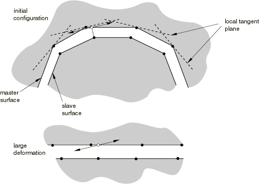
The basic guidelines given in “Defining contact pairs in Abaqus/Standard,” Section 34.3.1, should still be followed in a small-sliding simulation—the slave surface should be the more refined surface or the surface on the more deformable body. However, in a small-sliding simulation more thought must be given when defining the master surface. With small-sliding contact each slave node views the master surface as a flat surface, which can be significantly different than the true shape of the surface, even in the local region near the anchor point. In some cases the local tangent planes provide a good local approximation to the master surface in the initial configuration, but deformation and rotation of the master surface can reorient the local tangent planes such that they become a poor representation of the master surface. Figure 36.1.115 shows an example where distortion of the master surface results in such a situation.
This problem can be minimized to some extent by using a more refined mesh on the master surface, thus providing more element faces to control the motion of the tangent planes. Excessive mesh refinement should not be necessary since only small sliding should occur.As was mentioned before, the small-sliding tracking approach reduces to an infinitesimal-sliding tracking approach for geometrically linear analyses. Infinitesimal sliding assumes that both the relative motions of the surfaces and the absolute motions of the model remain small. The orientations of the local tangent planes are not updated, and the load transfer paths and the weightings assigned to each master surface node remain constant during an infinitesimal-sliding simulation.
As in the case of small sliding, you can choose between node-to-surface and surface-to-surface discretizations with the infinitesimal-sliding tracking approach. The same user interface applies, and the default is node-to-surface discretization.
Local tangent directions on a contact surface (sometimes called “slip directions”) are a reference orientation by which Abaqus calculates tangential behavior in a contact interaction. Abaqus/Standard calculates the initial orientation of the two local tangent directions by default. The local tangent directions rotate with the contact surface in a geometrically nonlinear analysis.
Two-dimensional and standard axisymmetric models have only one local tangent direction, ![]() . Abaqus/Standard defines the orientation of this direction by the cross product of the vector into the plane of the model (0., 0., 1.0) and the contact normal vector.
. Abaqus/Standard defines the orientation of this direction by the cross product of the vector into the plane of the model (0., 0., 1.0) and the contact normal vector.
Models consisting of generalized axisymmetric bodies have a second local tangent direction, ![]() , to account for the component of slip associated with relative differences in circumferential twist between contacting bodies. The first local tangent direction at any point on the surface is always tangent to the master surface in the local r–z plane. The second local tangent direction is orthogonal to this plane in the local circumferential direction. For more information about generalized axisymmetric models, see “Generalized axisymmetric stress/displacement elements with twist” in “Choosing the element's dimensionality,” Section 26.1.2.
, to account for the component of slip associated with relative differences in circumferential twist between contacting bodies. The first local tangent direction at any point on the surface is always tangent to the master surface in the local r–z plane. The second local tangent direction is orthogonal to this plane in the local circumferential direction. For more information about generalized axisymmetric models, see “Generalized axisymmetric stress/displacement elements with twist” in “Choosing the element's dimensionality,” Section 26.1.2.
By default, Abaqus/Standard determines the initial orientation of the two local tangent directions, ![]() and
and ![]() , using the following conventions:
, using the following conventions:
Finite-sliding, surface-to-surface formulation: The default initial orientations of the two local tangent directions are based on the slave surface normal, using the standard convention for calculating surface tangents (see “Conventions,” Section 1.2.2) with the assumption that the contact normal corresponds to the negative normal to the slave surface.
Finite-sliding, node-to-surface formulation: For contact involving a slave surface based on three-dimensional beam-type elements, the first and second local tangent directions are defined along the length of the beam and transverse to the beam, respectively. For contact involving an analytical rigid surface and a slave surface that is not based on three-dimensional beam-type elements, the first local tangent direction is tangential to the cross-section used to generate the analytical rigid surface, and the second local tangent direction is orthogonal to the plane of the cross-section in which the contact occurs.In other cases, default initial orientations of the two local tangent directions are calculated by first computing tentative ![]() and
and ![]() directions. For element-based slave surfaces the tentative directions are based on the slave surface using the standard convention for calculating surface tangents. For node-based slave surfaces the tentative
directions. For element-based slave surfaces the tentative directions are based on the slave surface using the standard convention for calculating surface tangents. For node-based slave surfaces the tentative ![]() and
and ![]() directions are set at each node to coincide with the global x- and y-axes, respectively. Abaqus constructs an orthogonal triad of
directions are set at each node to coincide with the global x- and y-axes, respectively. Abaqus constructs an orthogonal triad of ![]() ,
, ![]() , and
, and ![]() (where
(where ![]() ), then rotates this triad such that
), then rotates this triad such that ![]() becomes aligned with the master surface normal at the tracked point on the master surface.
becomes aligned with the master surface normal at the tracked point on the master surface.
Small-sliding, surface-to-surface formulation: The default initial orientations of the two local tangent directions are based on the slave surface normal, using the standard convention for calculating surface tangents, except for contact involving analytical rigid surfaces, in which case the local tangent directions are based on the master surface normal.
Small-sliding, node-to-surface formulation: The default initial orientations of the two local tangent directions are calculated at each point on the master surface based on the master surface normal, using the standard convention for calculating surface tangents.
If the default local tangent directions are not convenient to prescribe an anisotropic friction model or to view contact output, you can define the local tangent directions for three-dimensional contact pair surfaces. You cannot redefine the local tangent directions for the following types of surfaces:
Surfaces in a general contact domain
Analytical rigid surfaces
Two-dimensional surfaces
You define the local tangent directions by associating an orientation definition (see “Orientations,” Section 2.2.5) with a contact pair surface. You can assign an orientation only to one surface of a contact pair. The surface on which an orientation can be defined is the same surface on which the default orientation would be calculated (see the conventions given previously). For example, an orientation can be defined only on the slave surface in deformable versus deformable finite-sliding contact. If a second orientation is also given, an error message is issued. Therefore, it is not possible to redefine the local tangent directions for finite-sliding contact between a deformable slave surface and an analytical rigid surface.
An orientation that is defined on a slave surface of a contact pair that is generated from three-dimensional truss-type elements or from a list of nodes without rotational degree of freedoms will not be rotated if the slave surface undergoes finite motion. In this case a warning message is issued during input processing.
| Input File Usage: | *CONTACT PAIR, INTERACTION=interaction_property_name slave surface name, master surface name, orientation for slave surface slave surface name, master surface name, , orientation for master surface |
| Abaqus/CAE Usage: | You cannot define alternative local tangent directions for contact pairs in Abaqus/CAE. |
For geometrically nonlinear analyses the local tangent directions rotate with the surface on which these directions were initially calculated or redefined using an orientation definition as described above with the exception that the local tangent direction rotates with the master surface for the small-sliding, surface-to-surface formulation. These rotated local tangent directions are further rotated to ensure that the normal vector, computed using the cross product of the rotated local tangent directions, corresponds to the normal vector on the master surface when the slave node comes into contact.