Products: Abaqus/Standard Abaqus/AMS
This example demonstrates the following Abaqus features and techniques for frequency extraction and steady-state dynamic analysis:
using the automatic multi-level substructuring (AMS) eigensolver in the frequency extraction step along with residual modes;
projecting a global material structural damping operator during the frequency extraction step using the AMS eigensolver;
using the SIM-based steady-state dynamic analysis procedure with material structural damping; and
demonstrating the performance benefit of the SIM-based steady-state dynamic analysis procedure using the AMS eigensolver compared to the subspace-based steady-state dynamic analysis procedure with the Lanczos eigensolver.
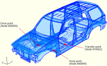
This example examines the structural behavior of a vehicle body-in-white (BIW) model in terms of eigenmodes and frequency response functions. In addition, this example demonstrates the use of the steady-state dynamic analysis procedure with the AMS eigensolver and the SIM architecture (see “Using the SIM architecture for modal superposition dynamic analyses” in “Dynamic analysis procedures: overview,” Section 6.3.1 of the Abaqus Analysis User's Manual) for an automobile structure. The model shown in Figure 2.2.6–1 was obtained from the National Highway Traffic Safety Administration (NHTSA) web site. This model includes material structural damping.
The primary goal of this example is to demonstrate the significant performance improvement of the SIM-based steady-state dynamic analysis procedure using the AMS eigensolver compared to the subspace-based steady-state dynamic analysis procedure. Prior to performing the steady-state dynamic analysis, the undamped eigensolution is computed using the AMS eigensolver. The global cutoff frequency of this model is 300 Hz, so the global eigenmodes below 300 Hz are extracted. During the reduction phase of the AMS eigensolver, all of the substructure eigenmodes below 1500 Hz are extracted and used to calculate the global eigensolution with the ![]() default value of 5. In addition, the material structural damping operator is projected onto the global eigenmode subspace.
default value of 5. In addition, the material structural damping operator is projected onto the global eigenmode subspace.
The model consists of the bare metal shell of the frame body including fixed windshields. This model has 127,213 elements and 794,292 active degrees of freedom, and a total of 1107 fasteners are defined to model spot welds in the frame body.
Linear elastic materials are used for all shell elements, and material structural damping with a value of 0.01 is applied to the materials for the ceiling, floor, hood, and side body of the vehicle. This type of damping results in a full system of modal equations that must be solved for each frequency point.
This structure is not constrained, so there are six rigid body modes in the model. Two concentrated loads are applied to the nodes at the two pivot points on the bottom of the vehicle floor to simulate the rolling motion of the vehicle in the steady-state dynamic analysis.
The objective of this analysis is an understanding of the overall structural response of a body-in-white model due to rolling motion. The response is evaluated by studying the frequency responses at both a drive point node and a transfer point node.
Compared to the subspace-based steady-state dynamic analysis procedure with the Lanczos eigensolver, the SIM-based steady-state dynamic analysis procedure using the AMS eigensolver shows significant performance benefit with acceptable accuracy. The accuracy of the SIM-based steady-state dynamic solution is evaluated by comparing the frequency response functions for the SIM-based and subspace-based steady-state dynamic analyses.
Drive point and transfer point responses are calculated at nodes 840950 and 874962, respectively, to demonstrate the accuracy of the SIM-based steady-state dynamic analysis procedure with eigenmodes computed by the AMS eigensolver. This model has 1210 global eigenmodes below the global cutoff frequency, including 6 rigid body modes. The AMS eigensolver approximates 1188 global eigenmodes below the global cutoff frequency of 300 Hz, and the frequency response solutions below 150 Hz are calculated at 1 Hz increments. Two residual modes are also added to demonstrate a means of improving efficiency by using fewer global modes.
The frequency extraction step is followed by a steady-state dynamic analysis step. The global cutoff frequency for the frequency extraction step is 300 Hz, and the frequency range considered is 1–150 Hz at 1 Hz increments. For the subspace-based steady-state dynamic analysis, 1000 eigenmodes below 300 Hz are used. For the SIM-based steady-state dynamic analysis, all the eigenmodes below 300 Hz (approximately 1200 eigenmodes) are used.
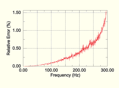
The accuracy of the natural frequencies computed by the AMS eigensolver is evaluated assuming that the natural frequencies computed by the Lanczos eigensolver are exact, and relative errors are shown in Figure 2.2.6–2. These errors are less than 1.6% at frequencies below the global cutoff frequency of 300 Hz. Below 150 Hz, the region of particular interest, the errors are less than 0.25% and the resonance peaks in the frequency response function are reasonably accurate.
The accuracy of the steady-state dynamics solutions is evaluated qualitatively by comparing the frequency response curves. The response curves are compared at two different output locations: a drive point node and a transfer point node.
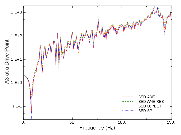
Figure 2.2.6–3 shows the point inertance at node 840950; the curve labeled SSD DIRECT represents the direct-solution steady-state dynamic analysis procedure, the curve labeled SSD SP represents the subspace-based steady-state dynamic analysis procedure, the curve labeled SSD AMS represents the SIM-based steady-state dynamic analysis procedure, and the curve labeled SSD AMS RES represents the SIM-based steady-state dynamic analysis procedure with residual modes. The curves are almost indistinguishable for frequencies below 125 Hz. To improve the accuracy of the response functions, residual modes can be added to compensate for high-frequency truncation errors. Calculation of residual modes is requested in the AMS eigenvalue extraction step by specifying the nodal points where forces are applied. For this solution (SSD AMS RES), the global cutoff frequency is set to 225 Hz instead of 300 Hz to demonstrate that the global cutoff frequency can be lowered without losing accuracy. By lowering the global cutoff frequency to 225 Hz and adding two residual modes in the global eigenmode subspace, a speed up of approximately 25% can be achieved.
Figure 2.2.6–4 shows the transfer inertance at the node located at the bottom of the driver’s seat; the same curve labels discussed above are used in this figure. The frequency response computed by the SIM-based steady-state dynamic analysis procedure nearly matches those computed by the subspace-based steady-state dynamic analysis procedure and the direct-solution steady-state dynamic analysis procedure for the frequencies below 125 Hz. To improve accuracy for frequencies higher than 125 Hz, more eigenmodes should be extracted and used.
The overall performance comparison among the three steady-state dynamic analysis procedures is summarized in Table 2.2.6–1 (analysis cost is independent of whether or not residual modes are used). Performance was evaluated on a Linux/x86-64 server with a single processor. The amount of available memory was set to 16 GB for each run. It is clear that the SIM-based steady-state dynamic analysis procedure using the AMS eigensolver shows excellent performance compared to the subspace-based steady-state dynamic analysis procedure using the Lanczos eigensolver or the direct-solution steady-state dynamic analysis procedure.
Input file for the BIW model data.
Frequency extraction analysis using the AMS eigensolver for the BIW model.
SIM-based steady-state dynamic analysis using the AMS eigensolution for the BIW model.
Frequency extraction analysis (including residual modes) using the AMS eigensolver for the BIW model.
SIM-based steady-state dynamic analysis using the AMS eigensolution including residual modes for the BIW model.
Frequency extraction analysis using the Lanczos eigensolver for the BIW model.
Subspace-based steady-state dynamic analysis using the Lanczos eigensolution for the BIW model.
Direct-solution steady-state dynamic analysis for the BIW model.
“Direct-solution steady-state dynamic analysis,” Section 6.3.4 of the Abaqus Analysis User's Manual
“Natural frequency extraction,” Section 6.3.5 of the Abaqus Analysis User's Manual
“Mode-based steady-state dynamic analysis,” Section 6.3.8 of the Abaqus Analysis User's Manual
“Subspace-based steady-state dynamic analysis,” Section 6.3.9 of the Abaqus Analysis User's Manual