Products: Abaqus/Standard Abaqus/Explicit
This example demonstrates the combined use of Abaqus/Standard and Abaqus/Explicit to provide a more cost effective solution than by using either Abaqus/Standard or Abaqus/Explicit alone. Abaqus features and techniques demonstrated include:
Abaqus/Standard to Abaqus/Explicit co-simulation, where
Abaqus/Standard employs substructuring, a feature not available in Abaqus/Explicit, to efficiently handle modeling of a component subjected to small strains, and
Abaqus/Explicit is used to efficiently simulate high-speed contact interactions.
This example considers the impact of a recreational scooter with a bump. An analysis of the transient response of an interaction with a bump is used to determine the accelerations felt by the scooter operator. With this analysis a product designer can make informed design decisions by varying certain design parameters, such as the frame component cross-section properties, tire material, or inflation pressure and observing their influence on the operator acceleration. Effective use of this simulation technique requires that the simulation turnaround time be as quick as possible while retaining essential fidelity in the results.
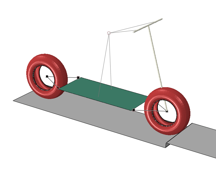
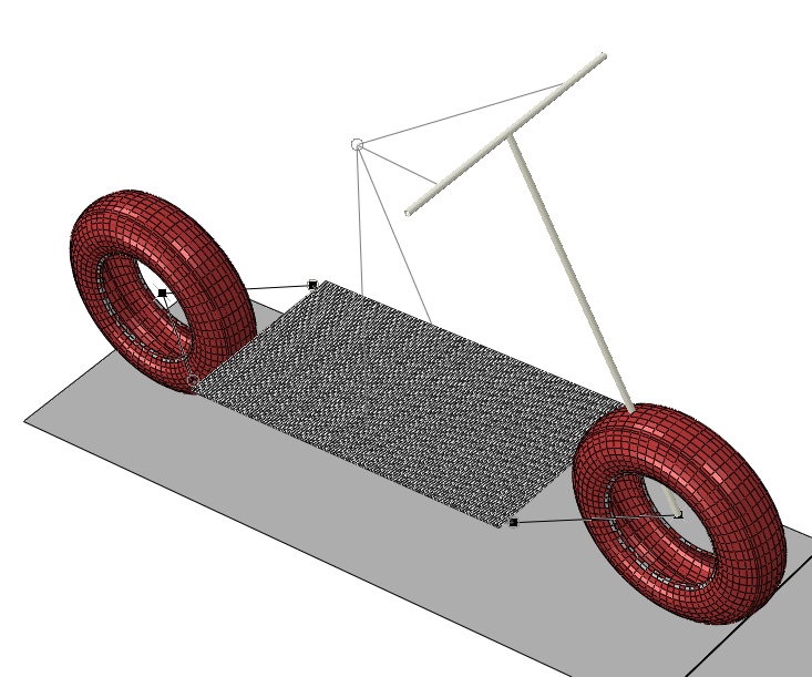
The scooter consists of an operator deck, a frame with handlebars, and two tires, as shown in Figure 2.4.2–1. The overall length of the scooter is 1200 mm, and the overall height is 800 mm. The handlebars are oriented straight.
The scooter deck and frame tubing are made of mild steel. The tires are a Butyl rubber material.
Several Abaqus analysis approaches can be used to simulate the transient behavior of the scooter: using only Abaqus/Standard, using only Abaqus/Explicit, or using Abaqus/Standard to Abaqus/Explicit co-simulation. To illustrate the computational cost savings of the co-simulation approach, the analysis cases that follow focus on comparing the co-simulation approach to an Abaqus/Explicit-only simulation approach.
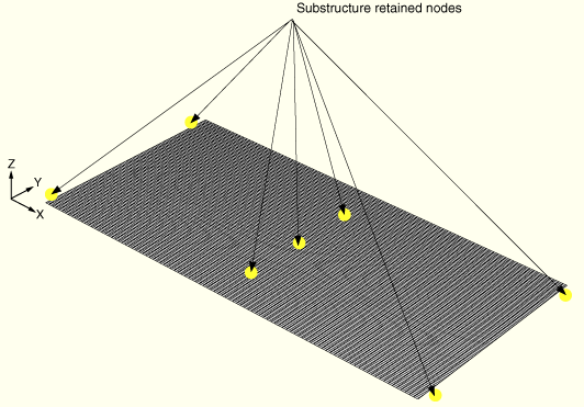
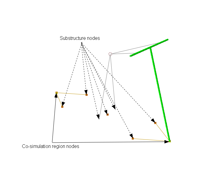
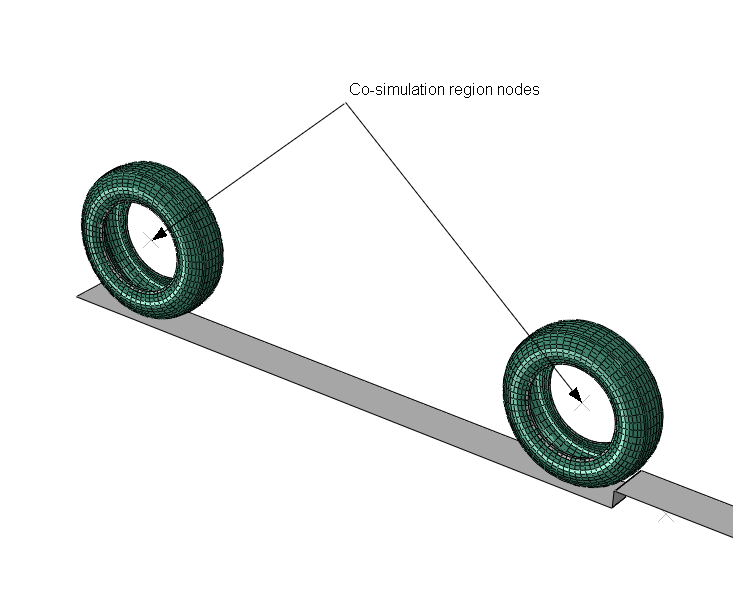
The Abaqus/Standard model of the co-simulation analysis consists of the scooter deck (Figure 2.4.2–2) and frame (Figure 2.4.2–3). The deck is modeled using substructure techniques to further reduce the solution cost. The Abaqus/Explicit model of the co-simulation analysis consists of the tires and the road with the bump (Figure 2.4.2–4). Co-simulation regions across which data will be exchanged during the co-simulation analysis are identified on each model at the location of the wheel axles.
| Case 1 | A reference analysis performed using only Abaqus/Explicit. |
| Case 2 | A co-simulation analysis using the subcyling coupling scheme. |
Both analysis cases address the same transient simulation.
The tire transient response and contact with the road are simulated using the explicit dynamics procedure. In Case 1 the explicit dynamics procedure applies to the rest of the model as well. The scooter frame transient response is simulated using the implicit dynamics procedure.
Static stabilization, substructuring, and import analysis techniques are used in this example.
The inflation of the tires uses the Abaqus/Standard static stabilization option.
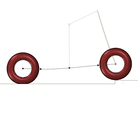
The meshed models are shown in Figure 2.4.2–5. The frame components are modeled using truss and connector elements. The deck is modeled using S4R shell elements. The tires are modeled using C3D8I continuum elements. The operator is represented by a point mass connected to foot and hand-hold locations through a distributing coupling constraint definition.
The deck is modeled as a simple linear elastic material, with an elastic modulus of 5 GPa, a Poisson's ratio of 0.3, and a density of 5000 kg/m3.
The tires are modeled as a hyperelastic material with viscoelastic properties. The tire material density is 1100 kg/m3.
An initial tire pressure of 20 KPa is applied. The tires begin the analysis in a statically equilibrated footprint configuration as a result of import from an earlier static analysis. The scooter is traveling toward the bump at an initial velocity of 3 m/s.
Forces are applied consistent with a total scooter weight of 42.4 N and a total operator weight of 222 N. To simplify the analysis setup, gravity loading is not applied; instead, the weight forces are applied at the axle locations. The main consequence of this loading approach is that the static sag of the deck due to the operator is neglected.
This analysis case uses Abaqus/Explicit exclusively for the transient analysis and is provided as a reference for comparing the results and computational cost of the co-simulation solution.
Abaqus/Explicit is used for the transient analysis with the tire inflation occurring using the static procedure in Abaqus/Standard.
In this case co-simulation occurs between Abaqus/Standard and Abaqus/Explicit, with each program advancing its simulation time according to its own automatic incrementation scheme and exchanging data as needed. Co-simulation data are exchanged at each Abaqus/Explicit time increment.
Abaqus/Explicit is used for the transient analysis of the tires with the tire inflation occurring using the static procedure in Abaqus/Standard. Abaqus/Standard is used for the transient analysis of the scooter frame and deck.
The following analysis step types are used.
An Abaqus/Standard static procedure is used to inflate the tires and establish the tire footprint.
The Abaqus/Explicit step does not employ mass scaling. The default bulk viscosity parameters are used.
The analyses in the co-simulation are run concurrently. The coupling identification between the analyses is achieved using the host and port parameters for the Abaqus execution procedure (see “Execution procedure for Abaqus/Standard and Abaqus/Explicit,” Section 3.2.2 of the Abaqus Analysis User's Manual).
For example, use the following commands to run the Abaqus/Standard job, establishing a co-simulation connection to an Abaqus/Explicit job running on a host named “abc” that is listening on port 48000:
abaqus analysis job=scooter_cosim_std host=abc port=48000
abaqus analysis job=scooter_cosim_xpl
   oldjob=scooter_tire_inflation port=48000
The results for a co-simulation analysis appear in multiple output files. To make effective use of the Abaqus/Standard and Abaqus/Explicit output databases, you should use the Abaqus/Viewer overlay functionality to view the combined results. For more information, see Chapter 75, “Overlaying multiple plots,” of the Abaqus/CAE User's Manual.
The results show that Case 1 is more computationally expensive. Case 2 provides a significant cost improvement. Further, the results show that the solution fidelity, when compared to the reference solution, is not significantly affected by the use of the co-simulation technique.
As the scooter collides with the bump, the entire assembly leaves the ground and flexes slightly, as shown in Figure 2.4.2–6.
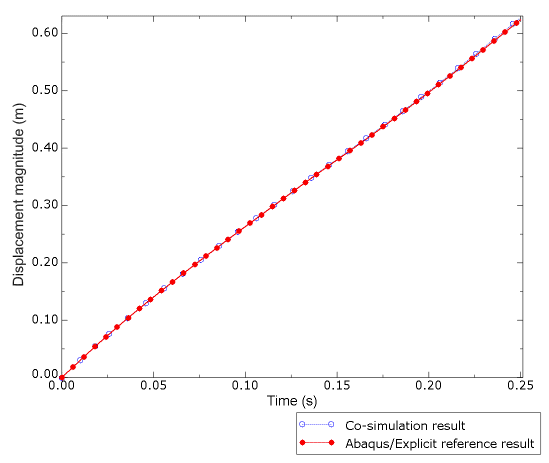
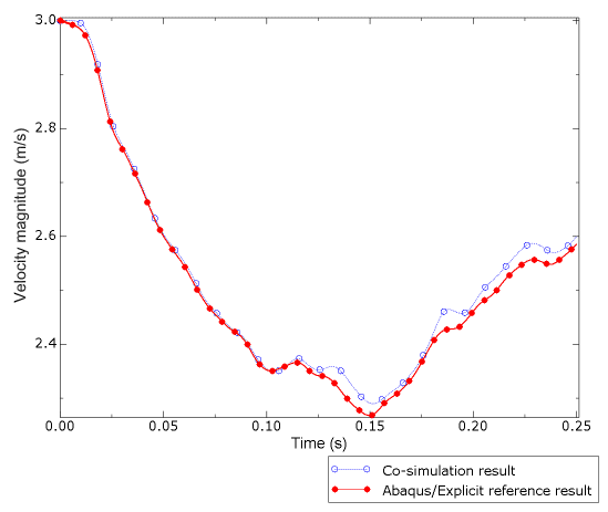
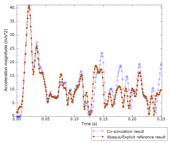
We consider measures of operator comfort to relate to the displacement, velocity, and acceleration magnitude histories at the operator node location. Figure 2.4.2–7, Figure 2.4.2–8, and Figure 2.4.2–9 show these respective response histories, comparing the results for the Case 1 and Case 2 analyses. The results are plotted after applying the Butterworth filter with a cut-off frequency of 100 Hz (see “Applying Butterworth filtering to an X–Y data object,” Section 43.4.26 of the Abaqus/CAE User's Manual, in the online HTML version of this manual), and show very good agreement between the Case 1 and Case 2 workflows.
Table 2.4.2–1 lists the relative computation cost of the two simulation approaches and clearly shows the value of co-simulation in this analysis.
Abaqus/Standard input file to inflate the tires and establish the static footprint due to the assembly weight.
Job parameters common to all scooter analyses.
Abaqus/Explicit input file to model all components, importing the inflated tires from scooter_tire_inflation.inp results and simulating the transient impact with the bump.
Tire and road modeling
Abaqus/Explicit input file to model the tires and road, importing the inflated tires from scooter_tire_inflation.inp results and simulating the transient impact with the bump through co-simulation coupling with scooter_cosim_std.inp.
Frame and deck modeling
Abaqus/Standard input file modeling the deck and creating the substructure representation of the deck.
Abaqus/Standard input file modeling the frame components, referring to the scooter_subgen.inp substructure definition and simulating the transient impact with the bump through co-simulation coupling with scooter_cosim_xpl.inp.
Table 2.4.2–1 Comparison of relative CPU times (normalized with respect to the CPU time for the Abaqus/Explicit analysis).
| Analysis job | Relative CPU time | |
|---|---|---|
| Co-simulation workflow | Abaqus/Explicit workflow | |
| Substructure generation | 0.007 | N/A |
| Tire inflation and footprint | 0.002 | 0.002 |
| Co-simulation Abaqus/Explicit analysis | 0.060 | N/A |
| Co-simulation Abaqus/Standard analysis | 0.057 | N/A |
| Complete Abaqus/Explicit analysis | N/A | 1.0 |
| Total simulation cost | 0.126 | 1.002 |