Products: Abaqus/Standard Abaqus/CAE Abaqus/Viewer
Modeling discontinuities, such as cracks, as an enriched feature:
is commonly referred to as the extended finite element method (XFEM);
is an extension of the conventional finite element method based on the concept of partition of unity;
allows the presence of discontinuities in an element by enriching degrees of freedom with special displacement functions;
does not require the mesh to match the geometry of the discontinuities;
is a very attractive and effective way to simulate initiation and propagation of a discrete crack along an arbitrary, solution-dependent path without the requirement of remeshing in the bulk materials;
can be simultaneously used with the surface-based cohesive behavior approach (see “Surface-based cohesive behavior,” Section 33.1.10) or the Virtual Crack Closure Technique (see “Crack propagation analysis,” Section 11.4.3), which are best suited for modeling interfacial delamination;
can also be used to perform contour integral evaluations for an arbitrary stationary surface crack without the need to refine the mesh around the crack tip;
allows contact interaction of cracked element surfaces based on a small-sliding formulation;
allows both material and geometrical nonlinearity; and
is currently available only for first-order stress/displacement solid continuum elements.
Modeling stationary discontinuities, such as a crack, with the conventional finite element method requires that the mesh conforms to the geometric discontinuities. Therefore, considerable mesh refinement is needed in the neighborhood of the crack tip to capture the singular asymptotic fields adequately. Modeling a growing crack is even more cumbersome because the mesh must be updated continuously to match the geometry of the discontinuity as the crack progresses.
The extended finite element method (XFEM) alleviates the shortcomings associated with meshing crack surfaces. The extended finite element method was first introduced by Belytschko and Black (1999). It is an extension of the conventional finite element method based on the concept of partition of unity by Melenk and Babuska (1996), which allows local enrichment functions to be easily incorporated into a finite element approximation. The presence of discontinuities is ensured by the special enriched functions in conjunction with additional degrees of freedom. However, the finite element framework and its properties such as sparsity and symmetry are retained.
For the purpose of fracture analysis, the enrichment functions typically consist of the near-tip asymptotic functions that capture the singularity around the crack tip and a discontinuous function that represents the jump in displacement across the crack surfaces. The approximation for a displacement vector function ![]() with the partition of unity enrichment is
with the partition of unity enrichment is
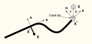
Figure 10.6.1–1 illustrates the asymptotic crack tip functions in an isotropic elastic material, ![]() , which are given by
, which are given by
![]()
These functions span the asymptotic crack-tip function of elasto-statics, and ![]() takes into account the discontinuity across the crack face. The use of asymptotic crack-tip functions is not restricted to crack modeling in an isotropic elastic material. The same approach can be used to represent a crack along a bimaterial interface, impinged on the bimaterial interface, or in an elastic-plastic power law hardening material. However, in each of these three cases different forms of asymptotic crack-tip functions are required depending on the crack location and the extent of the inelastic material deformation. The different forms for the asymptotic crack-tip functions are discussed by Sukumar (2004), Sukumar and Prevost (2003), and Elguedj (2006), respectively.
takes into account the discontinuity across the crack face. The use of asymptotic crack-tip functions is not restricted to crack modeling in an isotropic elastic material. The same approach can be used to represent a crack along a bimaterial interface, impinged on the bimaterial interface, or in an elastic-plastic power law hardening material. However, in each of these three cases different forms of asymptotic crack-tip functions are required depending on the crack location and the extent of the inelastic material deformation. The different forms for the asymptotic crack-tip functions are discussed by Sukumar (2004), Sukumar and Prevost (2003), and Elguedj (2006), respectively.
Accurately modeling the crack-tip singularity requires constantly keeping track of where the crack propagates and is cumbersome because the degree of crack singularity depends on the location of the crack in a non-isotropic material. Therefore, we consider the asymptotic singularity functions only when modeling stationary cracks in Abaqus/Standard. Moving cracks are modeled using the alternative approach described below.
The alternative approach within the framework of XFEM is based on traction-separation cohesive behavior. This approach is used in Abaqus/Standard to simulate crack initiation and propagation. The other crack initiation and propagation capabilities available in Abaqus/Standard are based on cohesive elements (“Defining the constitutive response of cohesive elements using a traction-separation description,” Section 29.5.6) or on surface-based cohesive behavior (“Surface-based cohesive behavior,” Section 33.1.10). Unlike these methods, which require that the cohesive surfaces align with element boundaries and the cracks propagate along a set of predefined paths, the XFEM-based cohesive segments method can be used to simulate crack initiation and propagation along an arbitrary, solution-dependent path in the bulk materials, since the crack propagation is not tied to the element boundaries in a mesh. In this case the near-tip asymptotic singularity is not needed, and only the displacement jump across a cracked element is considered. Therefore, the crack has to propagate across an entire element at a time to avoid the need to model the stress singularity.
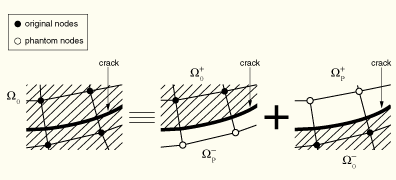
Phantom nodes, which are superposed on the original real nodes, are introduced to represent the discontinuity of the cracked elements, as illustrated in Figure 10.6.1–2. When the element is intact, each phantom node is completely constrained to its corresponding real node. When the element is cut through by a crack, the cracked element splits into two parts. Each part is formed by a combination of some real and phantom nodes depending on the orientation of the crack. Each phantom node and its corresponding real node are no longer tied together and can move apart.The magnitude of the separation is governed by the cohesive law until the cohesive strength of the cracked element is zero, after which the phantom and the real nodes move independently. To have a set of full interpolation bases, the part of the cracked element that belongs in the real domain, ![]() , is extended to the phantom domain,
, is extended to the phantom domain, ![]() . Then the displacement in the real domain,
. Then the displacement in the real domain, ![]() , can be interpolated by using the degrees of freedom for the nodes in the phantom domain,
, can be interpolated by using the degrees of freedom for the nodes in the phantom domain, ![]() . The jump in the displacement field is realized by simply integrating only over the area from the side of the real nodes up to the crack; i.e.,
. The jump in the displacement field is realized by simply integrating only over the area from the side of the real nodes up to the crack; i.e., ![]() and
and ![]() . This method provides an effective and attractive engineering approach and has been used for simulation of the initiation and growth of multiple cracks in solids by Song (2006) and Remmers (2008). It has been proven to exhibit almost no mesh dependence if the mesh is sufficiently refined.
. This method provides an effective and attractive engineering approach and has been used for simulation of the initiation and growth of multiple cracks in solids by Song (2006) and Remmers (2008). It has been proven to exhibit almost no mesh dependence if the mesh is sufficiently refined.
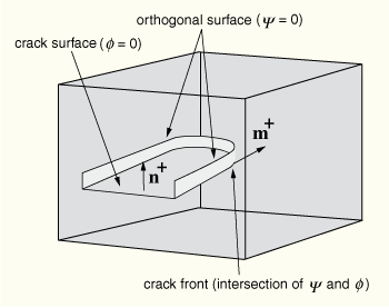
A key development that facilitates treatment of cracks in an extended finite element analysis is the description of crack geometry, because the mesh is not required to conform to the crack geometry. The level set method, which is a powerful numerical technique for analyzing and computing interface motion, fits naturally with the extended finite element method and makes it possible to model arbitrary crack growth without remeshing. The crack geometry is defined by two almost-orthogonal signed distance functions, as illustrated in Figure 10.6.1–3. The first, ![]() , describes the crack surface, while the second,
, describes the crack surface, while the second, ![]() , is used to construct an orthogonal surface so that the intersection of the two surfaces gives the crack front.
, is used to construct an orthogonal surface so that the intersection of the two surfaces gives the crack front. ![]() indicates the positive normal to the crack surface;
indicates the positive normal to the crack surface; ![]() indicates the positive normal to the crack front. No explicit representation of the boundaries or interfaces is needed because they are entirely described by the nodal data. Two signed distance functions per node are generally required to describe a crack geometry.
indicates the positive normal to the crack front. No explicit representation of the boundaries or interfaces is needed because they are entirely described by the nodal data. Two signed distance functions per node are generally required to describe a crack geometry.
You must specify an enriched feature and its properties. One or multiple pre-existing cracks can be associated with an enriched feature. In addition, during an analysis one or multiple cracks can initiate in an enriched feature without any initial defects. Enriched degrees of freedom are activated only when an element is intersected by a crack. Only stress/displacement solid continuum elements can be associated with an enriched feature.
| Input File Usage: | *ENRICHMENT |
| Abaqus/CAE Usage: | Interaction module: Special |
You can choose to model discrete crack propagation along an arbitrary, solution-dependent path or an arbitrary stationary crack. The former infers that crack propagation is modeled with the cohesive segments method in conjunction with phantom nodes. The latter requires that the elements around the crack tips are enriched with asymptotic functions to catch the singularity and that the elements intersected by the crack interior are enriched with the jump function across the crack surfaces. However, the options are mutually exclusive and cannot be specified simultaneously in a model.
| Input File Usage: | Use the following option to specify a crack propagation analysis (default): |
*ENRICHMENT, TYPE=PROPAGATION CRACK Use the following option to specify an analysis with stationary cracks: *ENRICHMENT, TYPE=STATIONARY CRACK |
| Abaqus/CAE Usage: | Use the following input to specify a crack propagation analysis: |
Interaction module: crack editor: toggle on Allow crack growth Use the following input to specify an analysis with stationary cracks: Interaction module: crack editor: toggle off Allow crack growth |
You must assign a name to an enriched feature, such as a crack. This name can be used in defining the initial location of the crack surfaces, in identifying a crack for contour integral output, and in activating or deactivating the crack propagation analysis.
| Input File Usage: | *ENRICHMENT, NAME=name |
| Abaqus/CAE Usage: | Interaction module: Special |
You must associate the enrichment definition with a region of your model. Only degrees of freedom in elements within these regions are potentially enriched with special functions. The region should consist of elements that are presently intersected by cracks and those that are likely to be intersected by cracks as the cracks propagate.
| Input File Usage: | *ENRICHMENT, ELSET=element set name |
| Abaqus/CAE Usage: | Interaction module: Special |
When an element is cut by a crack, the compressive behavior of the crack surfaces has to be considered. The formulae that govern behavior are very similar to those used for surface-based small-sliding penalty contact (“Mechanical contact properties: overview,” Section 33.1.1). However, the frictional behavior is not yet considered in the shear direction.
For an element intersected by a stationary crack, it is assumed that the elastic cohesive strength of the cracked element is zero. Therefore, compressive behavior of the crack surfaces is fully defined with the above options when the crack surfaces come into contact. For a moving crack, the situation is more complex; traction-separation cohesive behavior as well as compressive behavior of the crack surfaces are involved in a cracked element. In the contact normal direction, the pressure-overclosure relationship governing the compressive behavior between the surfaces does not interact with the cohesive behavior, since they each describe the interaction between the surfaces in a different contact regime. The pressure-overclosure relationship governs the behavior only when the crack is “closed”; the cohesive behavior contributes to the contact normal stress only when the crack is “open” (i.e., not in contact).
If the elastic cohesive stiffness of an element is undamaged in the shear direction, it is assumed that the cohesive behavior is active. Any tangential slip is assumed to be purely elastic in nature and is resisted by the elastic cohesive strength of the element, resulting in shear forces. If damage has been defined, the cohesive contribution to the shear stresses starts degrading with damage evolution. Once maximum degradation has been reached, the cohesive contribution to the shear stresses is zero.
| Input File Usage: | Use the following options to define contact of crack surfaces using a small-sliding formulation: |
*ENRICHMENT, INTERACTION=interaction_property_name *SURFACE INTERACTION, NAME=interaction_property_name *SURFACE BEHAVIOR, PENALTY=LINEAR |
| Abaqus/CAE Usage: | Interaction module: crack editor: toggle on Specify contact property |
The formulae and laws that govern the behavior of XFEM-based cohesive segments for a crack propagation analysis are very similar to those used for cohesive elements with traction-separation constitutive behavior (“Defining the constitutive response of cohesive elements using a traction-separation description,” Section 29.5.6) and those used for surface-based cohesive behavior (“Surface-based cohesive behavior,” Section 33.1.10). The similarities extend to the linear elastic traction-separation model, damage initiation criteria, and damage evolution laws.
The available traction-separation model in Abaqus assumes initially linear elastic behavior followed by the initiation and evolution of damage. The elastic behavior is written in terms of an elastic constitutive matrix that relates the normal and shear stresses to the normal and shear separations of a cracked element.
The nominal traction stress vector, ![]() , consists of the following components:
, consists of the following components: ![]() ,
, ![]() , and (in three-dimensional problems)
, and (in three-dimensional problems) ![]() , which represent the normal and the two shear tractions, respectively. The corresponding separations are denoted by
, which represent the normal and the two shear tractions, respectively. The corresponding separations are denoted by ![]() ,
, ![]() , and
, and ![]() . The elastic behavior can then be written as
. The elastic behavior can then be written as
The normal and tangential stiffness components will not be coupled: pure normal separation by itself does not give rise to cohesive forces in the shear directions, and pure shear slip with zero normal separation does not give rise to any cohesive forces in the normal direction.
The terms ![]() ,
, ![]() , and
, and ![]() are calculated based on the elastic properties for an enriched element. Specifying the elastic properties of the material in an enriched region is sufficient to define both the elastic stiffness and the traction-separation behavior.
are calculated based on the elastic properties for an enriched element. Specifying the elastic properties of the material in an enriched region is sufficient to define both the elastic stiffness and the traction-separation behavior.
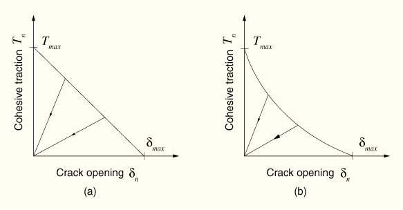
Damage modeling allows you to simulate the degradation and eventual failure of an enriched element. The failure mechanism consists of two ingredients: a damage initiation criterion and a damage evolution law. The initial response is assumed to be linear as discussed in the previous section. However, once a damage initiation criterion is met, damage can occur according to a user-defined damage evolution law. Figure 10.6.1–4 shows a typical linear and a typical nonlinear traction-separation response with a failure mechanism. The enriched elements do not undergo damage under pure compression.
Damage of the traction-separation response for cohesive behavior in an enriched element is defined within the same general framework used for conventional materials (see “Progressive damage and failure,” Section 21.1.1). However, unlike cohesive elements with traction-separation behavior, you do not have to specify the undamaged traction-separation behavior in an enriched element.
Crack initiation refers to the beginning of degradation of the cohesive response at an enriched element. The process of degradation begins when the stresses or the strains satisfy specified crack initiation criteria. Two crack initiation criteria are available, based on the maximum principal stress or the maximum principal strain. An additional crack orthogonal to the maximum principal stress/strain direction is introduced when the fracture criterion, f, after each equilibrium increment reaches the value 1.0 within a given tolerance:
![]()
| Input File Usage: | *DAMAGE INITIATION, TOLERANCE= |
| Abaqus/CAE Usage: | Property module: material editor: Mechanical: Damage for Traction Separation Laws: Maxpe Damage or Maxps Damage: Tolerance: |
The maximum principal stress criterion can be represented as
![]()
| Input File Usage: | *DAMAGE INITIATION, CRITERION=MAXPS |
| Abaqus/CAE Usage: | Property module: material editor: Mechanical: Damage for Traction Separation Laws: Maxps Damage |
The maximum principal strain criterion can be represented as
![]()
| Input File Usage: | *DAMAGE INITIATION, CRITERION=MAXPE |
| Abaqus/CAE Usage: | Property module: material editor: Mechanical: Damage for Traction Separation Laws: Maxpe Damage |
The damage evolution law describes the rate at which the cohesive stiffness is degraded once the corresponding initiation criterion is reached. The general framework for describing the evolution of damage is conceptually similar to that used for damage evolution in surface-based cohesive behavior (“Surface-based cohesive behavior,” Section 33.1.10).
A scalar damage variable, D, represents the overall damage at the intersection between the surfaces of cracked elements. It initially has a value of 0. If damage evolution is modeled, D monotonically evolves from 0 to 1 upon further loading after the initiation of damage. The normal and shear stress components are affected by the damage according to
![]()
![]()
![]()
To describe the evolution of damage under a combination of normal and shear separations across the interface, an effective separation is defined as
![]()
| Input File Usage: | Use the following option to specify a damage evolution law: |
*DAMAGE EVOLUTION |
| Abaqus/CAE Usage: | Property module: material editor: Mechanical |
Models exhibiting various forms of softening behavior and stiffness degradation often lead to severe convergence difficulties in Abaqus/Standard. Viscous regularization of the constitutive equations defining cohesive behavior in an enriched element can be used to overcome some of these convergence difficulties. Viscous regularization damping causes the tangent stiffness matrix to be positive definite for sufficiently small time increments.
The approximate amount of energy associated with viscous regularization over the whole model is available using output variable ALLCD.
| Input File Usage: | Use the following option to specify viscous regularization: |
*DAMAGE STABILIZATION |
| Abaqus/CAE Usage: | Property module: material editor: Mechanical |
Because the mesh is not required to conform to the geometric discontinuities, the initial location of a pre-existing crack must be specified in the model. The level set method is provided for this purpose. Two signed distance functions per node are generally required to describe a crack geometry. The first describes the crack surface, while the second is used to construct an orthogonal surface so that the intersection of the two surfaces gives the crack front (see “Initial conditions,” Section 30.2.1).
The first signed distance function must be either greater or less than zero and cannot be equal to zero. If an initial crack has to be defined at the boundaries of an element, a very small positive or negative value for the first signed distance function must be specified.
| Input File Usage: | Use the following option to specify the initial location of an enriched feature: |
*INITIAL CONDITIONS, TYPE=ENRICHMENT |
| Abaqus/CAE Usage: | Interaction module: crack editor: Crack location: Select: select region |
The crack propagation capability can be activated or deactivated within the step definition.
| Input File Usage: | Use the following option to activate the crack propagation capability within the step definition: |
*ENRICHMENT ACTIVATION, NAME=name, ACTIVATE=ON (default) Use the following option to deactivate the crack propagation capability within the step definition: *ENRICHMENT ACTIVATION, NAME=name, ACTIVATE=OFF |
| Abaqus/CAE Usage: | To modify the status of the crack propagation capability in a step, you must first create an XFEM crack growth interaction: |
Interaction module: Create Interaction: select initial step: XFEM Crack Growth: select crack: Interaction manager: select interaction in step: Edit: toggle on/off Allow crack growth in this step |
When you evaluate the contour integrals using the conventional finite element method (“Contour integral evaluation,” Section 11.4.2 ) , you must define the crack front explicitly and specify the virtual crack extension direction in addition to matching the mesh to the cracked geometry. Detailed focused meshes are generally required and obtaining accurate contour integral results for a crack in a three-dimensional curved surface can be cumbersome. The extended finite element in conjunction with the level set method alleviates these shortcomings. The adequate singular asymptotic fields and the discontinuity are ensured by the special enriched functions in conjunction with additional degrees of freedom. In addition, the crack front and the virtual crack extension direction are determined automatically by the level set signed distance functions.
| Input File Usage: | Use the following option to obtain contour integral for a named enriched feature with the extended finite element method: |
*CONTOUR INTEGRAL, XFEM, CRACK NAME=name |
| Abaqus/CAE Usage: | Step module: history output request editor: Domain: Crack: crack name |
Although XFEM has alleviated the shortcomings associated with refining the mesh in the neighborhood of the crack front due to the added asymptotic fields, you must generate a sufficient number of elements around the crack front to obtain path-independent contours. The group of elements within a small radius from the crack front are enriched and become involved in the contour integral calculations. The default enrichment radius is three times the typical element characteristic length in the enriched area. You must include the elements inside the enrichment radius in the element set used to define the enriched region.
| Input File Usage: | Use the following option to specify an enrichment radius: |
*ENRICHMENT, ENRICHMENT RADIUS |
| Abaqus/CAE Usage: | Interaction module: crack editor: Enrichment radius: Analysis default or Specify |
Modeling discontinuities as an enriched feature can be performed using the static procedure (see “Static stress analysis,” Section 6.2.2).
Initial conditions to identify initial boundaries or interfaces of an enriched feature can be specified (see “Initial conditions,” Section 30.2.1).
Boundary conditions can be applied to any of the displacement degrees of freedom (see “Boundary conditions,” Section 30.3.1).
The following types of loading can be prescribed in a model with an enriched feature:
Concentrated nodal forces can be applied to the displacement degrees of freedom (1–3); see “Concentrated loads,” Section 30.4.2.
Distributed pressure forces or body forces can be applied; see “Distributed loads,” Section 30.4.3. The distributed load types available with particular elements are described in Part VI, “Elements.”
The following predefined fields can be specified in a model with an enriched feature, as described in “Predefined fields,” Section 30.6.1:
Although temperature is not a degree of freedom in stress/displacement elements, nodal temperatures can be specified as predefined fields. The specified temperature affects temperature-dependent critical stress and strain failure criteria, if specified.
The values of user-defined field variables can be specified. These values affect field-variable-dependent material properties, if specified.
Any of the mechanical constitutive models in Abaqus/Standard can be used to model the mechanical behavior of the enriched element. See Part V, “Materials.” The inelastic definition in a material point must be used in conjunction with the linear elastic material model (“Linear elastic behavior,” Section 19.2.1), the porous elastic material model (“Elastic behavior of porous materials,” Section 19.3.1), or the hypoelastic material model (“Hypoelastic behavior,” Section 19.4.1).
Only first-order solid continuum stress/displacement elements can be associated with an enriched feature. For propagating cracks these include bilinear plane strain and plane stress elements, linear brick elements, and linear tetrahedron elements. For stationary cracks, these include linear brick and linear tetrahedron elements.
In addition to the standard output identifiers available in Abaqus (“Abaqus/Standard output variable identifiers,” Section 4.2.1), the following variables have special meaning for a model with an enriched feature:
PHILSM | Signed distance function to describe the crack surface. |
PSILSM | Signed distance function to describe the initial crack front. |
STATUSXFEM | Status of the enriched element. (The status of an enriched element is 1.0 if the element is completely cracked and 0.0 if the element contains no crack. If the element is partially cracked, the value of STATUSXFEM lies between 1.0 and 0.0.) |
The following limitations exist with an enriched feature:
An enriched element cannot be intersected by more than one crack.
A crack is not allowed to turn more than 90° in one increment during an analysis.
Only asymptotic crack-tip fields in an isotropic elastic material are considered for a stationary crack.
Element loop operations are not yet supported in parallel execution mode.
The following is an example of modeling crack propagation with the extended finite element method:
*HEADING
...
*NODE, NSET=ALL
...
*ELEMENT, TYPE=C3D8, ELSET=REGULAR
*ELEMENT, TYPE=C3D8, ELSET=ENRICHED
...
*SOLID SECTION, MATERIAL=STEEL1, ELSET=REGULAR
*SOLID SECTION, MATERIAL=STEEL12, ELSET=ENRICHED

*ENRICHMENT, TYPE=PROPAGATION CRACK, ELSET=ENRICHED,
NAME=ENRICHMENT, INTERACTION=INTERACTION
*MATERIAL,NAME=STEEL1
...
*MATERIAL,NAME=STEEL2
*DAMAGE INITIATION, CRITERION=MAXPS, TOLERANCE=0.05
*DAMAGE EVOLUTION, TYPE=ENERGY
Data lines to specify the failure mechanism
...
*SURFACE INTERACTION, NAME=INTERACTION
*SURFACE BEHAVIOR
Data lines to specify the contact of cracked element surfaces
...
*STEP
*STATIC
...
*END STEP
*STEP
*STATIC
...

*ENRICHMENT ACTIVATION, TYPE=PROPAGATION CRACK,
NAME=ENRICHMENT, ACTIVATE=OFF
...
*END STEP
The following is an example of calculating contour integrals in stationary cracks with the extended finite element method:
*HEADING
...
*NODE, NSET=ALL
...
*ELEMENT, TYPE=C3D8, ELSET=REGULAR
*ELEMENT, TYPE=C3D8, ELSET=ENRICHED
...
*SOLID SECTION, MATERIAL=STEEL1, ELSET=REGULAR
*SOLID SECTION, MATERIAL=STEEL12, ELSET=ENRICHED

*ENRICHMENT, TYPE=STATIONARY CRACK, ELSET=ENRICHED,
NAME=ENRICHMENT, ENRICHMENT RADIUS
*MATERIAL,NAME=STEEL1
...
*MATERIAL,NAME=STEEL2
...
*STEP
*STATIC
...
*CONTOUR INTEGRAL,CRACK NAME=ENRICHMENT,XFEM
*END STEP
Belytschko, T., and T. Black, “Elastic Crack Growth in Finite Elements with Minimal Remeshing,” International Journal for Numerical Methods in Engineering, vol. 45, pp. 601–620, 1999.
Elguedj, T., A. Gravouil, and A. Combescure, “Appropriate Extended Functions for X-FEM Simulation of Plastic Fracture Mechanics,” Computer Methods in Applied Mechanics and Engineering, vol. 195, pp. 501–515, 2006.
Melenk, J., and I. Babuska, “The Partition of Unity Finite Element Method: Basic Theory and Applications,” Computer Methods in Applied Mechanics and Engineering, vol. 39, pp. 289–314, 1996.
Remmers, J. J. C., R. de Borst, and A. Needleman, “The Simulation of Dynamic Crack Propagation using the Cohesive Segments Method,” Journal of the Mechanics and Physics of Solids, vol. 56, pp. 70–92, 2008.
Song, J. H., P. M. A. Areias, and T. Belytschko, “A Method for Dynamic Crack and Shear Band Propagation with Phantom Nodes,” International Journal for Numerical Methods in Engineering, vol. 67, pp. 868–893, 2006.
Sukumar, N., Z. Y. Huang, J.-H. Prevost, and Z. Suo, “Partition of Unity Enrichment for Bimaterial Interface Cracks,” International Journal for Numerical Methods in Engineering, vol. 59, pp. 1075–1102, 2004.
Sukumar, N., and J.-H. Prevost, “Modeling Quasi-Static Crack Growth with the Extended Finite Element Method Part I: Computer Implementation,” International Journal for Solids and Structures, vol. 40, pp. 7513–7537, 2003.