The co-simulation technique is a multiphysics capability that provides several functions, available within Abaqus or as separate add-on analysis capabilities, for run-time coupling of Abaqus and another analysis program. An Abaqus analysis can be coupled to another Abaqus analysis or to a third-party analysis program to perform multidisciplinary simulations and multidomain (multimodel) coupling.
Abaqus provides built-in procedures to solve multidisciplinary simulations as described in “Multiphysics analyses” in “Procedures: overview,” Section 6.1.1. For multidisciplinary problems for which Abaqus does not provide a built-in solution procedure or where the solution procedure is limited in functionality, you can use the co-simulation technique to couple Abaqus with a third-party analysis program; for example, fluid-structure interaction (FSI) simulation in conjunction with computational fluid dynamics (CFD) analysis programs.
Another application area is solving complex problems where the model is divided into multiple domains and different analysis programs are used to obtain solutions for each domain; for example, crash safety simulation performed in conjunction with the occupant simulation program MADYMO.
Another example of this multiple domain analysis approach is with Abaqus/Standard to Abaqus/Explicit co-simulation, where each Abaqus analysis operates on a complementary section of the model domain where it is expected to provide the more computationally efficient solution. For example, Abaqus/Standard provides a more efficient solution for light and stiff components, while Abaqus/Explicit is more efficient for solving complex contact interactions.
The Abaqus co-simulation technique:
can be used to solve complex fluid-structure interactions by coupling Abaqus with CFD analysis programs;
can be used for crash safety simulations by coupling Abaqus/Explicit with the occupant simulation program MADYMO;
can be used for multidisciplinary simulations by coupling Abaqus with third-party analysis programs or in-house codes;
can be used to solve complex analyses more effectively by coupling Abaqus/Standard to Abaqus/Explicit; and
is intended for advanced users with in-depth knowledge of Abaqus and the third-party analysis program.
In a co-simulation the interaction between the domains is through a common physical interface over which data are exchanged in a synchronized manner between Abaqus and the coupled analysis program.
One domain may affect the response of another domain through one or more of the following:
the constitutive behavior, such as the yield stress defined as a function of temperature or stress defined as a function of other solution fields, such as thermal strains or the piezoelectric effect;
surface tractions/fluxes, such as a fluid exerting pressure on a structure;
body forces/fluxes, such as heat generation due to flow of current in a coupled thermal-electrical simulation;
contact forces, such as the forces due to contact between a vehicle and an occupant/pedestrian modeled as separate domains; and
geometric changes, such as fluid in contact with a deforming structure.
Fluid-structure interaction (FSI) covers a very broad scope of problems in which fluid flow and structural deformation interact and affect one another. The interaction can be mechanical, thermal, or both. Examples of FSI applications include hemodynamics in an artery, fluid flow in a pump, airflow over an aircraft wing, heat exchange in a radiator, heat transfer in turbine discs, fluid sloshing in a tank, and hydroplaning of a tire. The use of the co-simulation capability to perform an FSI simulation is illustrated in “Closure of an air-filled door seal,” Section 2.4.1 of the Abaqus Example Problems Manual.
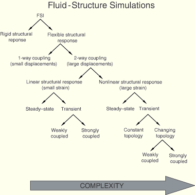
Figure 14.1.1–1 classifies FSI problems. The complexity of the simulation increases from left to right. At the uppermost level one can distinguish between rigid and flexible structural response problems. Rigid structural response problems are effectively handled by most computational fluid dynamics analysis programs; thus, an Abaqus co-simulation need be employed only for flexible structures.
In some cases the coupling strength (influence coefficient) in one direction may be so small as to be negligible (e.g., mechanical response influence on a fluid for a small-deformation analysis). These cases permit the use of a sequential analysis or a “unidirectional” co-simulation, where loads are passed from one analysis program to another analysis program but not vice versa.
The co-simulation interface allows for both unidirectional (MpCCI only) and bidirectional transfer of data. The structural response may be linear or nonlinear for material and geometric effects. Both steady-state and transient simulations are supported.
For fluid-structure interaction, Abaqus offers two approaches to couple with popular CFD solvers:
Coupling through the Mesh-based parallel Code Coupling Interface (MpCCI), a third-party connectivity approach for general multidisciplinary co-simulation.
Coupling directly with the AcuSolve general-purpose finite element flow solver.
The Mesh-based parallel Code Coupling Interface (MpCCI) developed and distributed by the Fraunhofer-Institute for Algorithms and Scientific Computing (SCAI) provides an open system approach for general multidisciplinary simulations between Abaqus and any third-party analysis program that supports MpCCI. MpCCI provides a scalable communication infrastructure and mapping algorithms for multiple physics domains. In a co-simulation using MpCCI, Abaqus communicates in real time with the MpCCI coupling server to exchange solution quantities with the third-party analysis program while each analysis advances its simulation time.
Coupling through MpCCI may occur between Abaqus and any third-party analysis program that supports the MpCCI interface. This includes in-house codes that have the MpCCI adapter embedded. SIMULIA actively supports and qualifies a link between Abaqus and STAR-CD and between Abaqus and FLUENT for fluid-structure interaction. For more information, refer to the Abaqus User's Guide for Fluid-Structure Interaction Using Abaqus and MpCCI.
The co-simulation technique allows coupling between Abaqus and AcuSolve, a general-purpose finite element flow solver. Both solvers communicate directly without any third-party communication tool.
The coupling between Abaqus and AcuSolve is actively supported and qualified by both SIMULIA and ACUSIM Software, Inc. For more information, refer to the Abaqus User's Guide for Fluid-Structure Interaction Using Abaqus and AcuSolve.
In certain cases you can realize significant computational cost savings by partitioning a model and combining the Abaqus/Standard and Abaqus/Explicit solutions, such as
when the simulation is principally a candidate for Abaqus/Explicit, but where certain parts of the model can be idealized using substructures in Abaqus/Standard, or
when the simulation is principally a candidate for Abaqus/Standard, but where complex contact conditions would be handled more effectively by Abaqus/Explicit.
Crash safety simulation generally includes interaction between a vehicle and its occupant or a vehicle and a pedestrian. Abaqus/Explicit is used to model the vehicle, and MADYMO is used to model the occupant or the pedestrian.
In some cases the influence of the human response on the structural response of the vehicle is so small as to be negligible. In these cases only a part of the vehicle surrounding the human is used in a coupled analysis. The vehicle analysis is performed without the human, and the motion from a portion of the vehicle immediately surrounding the human is extracted as a submodel of the full vehicle response. The co-simulation technique is used to perform a coupled analysis with the human model and the vehicle submodel.
The coupling between Abaqus/Explicit and MADYMO is actively supported and tested by both SIMULIA and TNO MADYMO BV.
You will typically apply co-simulation techniques to problems where the most complex physics occurs within domains that are handled exclusively within an analysis program (e.g., Abaqus or a CFD analysis program). Due to the comparative numerical simplicity of the numerical techniques applied at the co-simulation interface, the physics controlling the interaction at the interface of the separate analysis domains (the strength of the physics coupling) must be relatively weak for the co-simulation technique to be applied effectively.
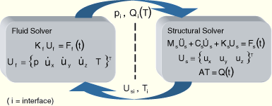
In a fluid-structure interaction (FSI) co-simulation the analysis domains are coupled in a staggered approach; that is, the equations for each domain are solved separately, and loads and boundary conditions are exchanged at the common interface. In mathematical terms the interaction is through the “right-hand side” only, as depicted in Figure 14.1.1–2, for the example of FSI co-simulation.
In an FSI co-simulation the flow equations are solved by the computational fluid dynamics analysis programs, and the structural equilibrium equations and heat transfer equations are solved by Abaqus. Only the loads and boundary conditions at the interface are exchanged during the simulation.Similarly, in a crash safety simulation with the vehicle modeled in Abaqus/Explicit and the dummy modeled in MADYMO, the interaction of the domains is resolved by application of the forces resulting from the contact condition between the interface of the two domains.
The staggered approach is applicable to many problems that exhibit weak to moderate physics coupling. In cases where the coupling is sufficiently weak, the coupling may be required only in one direction (such as when a temperature field contributes to the structural response, but a reverse coupling provides no significant impact on the simulation results).
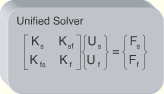
The staggered approach may not be effective for problems that exhibit strong physics coupling. In such cases it is best to solve the problem with dedicated analysis programs in which the solutions of all domains are combined into a single system and solved simultaneously (see Figure 14.1.1–3). Such solution approaches have their own numerical challenges and are not suited for general-purpose analysis programs such as Abaqus.
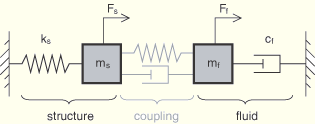
Figure 14.1.1–4 illustrates the coupling strength with an analogy in the frequency domain. Consider a lumped parameter dynamic system with a coupling impedance directly related to a response frequencyThe strength of the physics coupling can generally be greater in the coupling of Abaqus/Standard to Abaqus/Explicit using the co-simulation technique. Through communication of “right-hand-side” and “left-hand-side” terms, Abaqus/Standard to Abaqus/Explicit co-simulation provides a robust interface solution across a wide range of problem parameters. In many cases you can choose to have Abaqus/Standard and Abaqus/Explicit each advance their solutions according to their own automatic time incrementation scheme without adversely affecting the interface solution stability.
Performing a multidisciplinary analysis using the co-simulation technique involves the following steps:
Preparing the Abaqus analysis for co-simulation (see “Preparing an Abaqus analysis for co-simulation,” Section 14.1.2).
For Abaqus/Standard to Abaqus/Explicit co-simulation, see “Performing an Abaqus/Standard to Abaqus/Explicit co-simulation,” Section 14.1.3.
For co-simulation using MpCCI or coupling Abaqus and AcuSolve, see “Performing a co-simulation using MpCCI or coupling Abaqus and AcuSolve,” Section 14.1.4.
Preparing the third-party analysis program for co-simulation:
For fluid-structure interaction simulations, see the Abaqus User's Guide for Multiphysics Simulation Using Abaqus and MpCCI and the Abaqus User's Guide for Fluid-Structure Interaction Using Abaqus and AcuSolve.
For crash safety simulations, see the Abaqus User's Guide for Crash Safety Simulation Using Abaqus/Explicit and MADYMO.
For the latest support information and useful tips on running FSI simulations and crash safety simulations, refer to the Answers available in the SIMULIA Online Support System (SOSS), which is accessible through the My Support section of www.simulia.com. The following documents are available in the SIMULIA Online Support System:
The Abaqus User's Guide for Multiphysics Simulation Using Abaqus and MpCCI is available from Answer 2420.
The Abaqus User's Guide for Fluid-Structure Interaction Using Abaqus and AcuSolve is available from Answer 3253.
The Abaqus User's Guide for Crash Safety Simulation Using Abaqus/Explicit and MADYMO is available from Answer 2721.