Products: Abaqus/Standard Abaqus/CAE
“Heat transfer analysis procedures: overview,” Section 6.5.1
“Defining a cavity radiation interaction,” Section 15.13.16 of the Abaqus/CAE User's Manual
“Defining a cavity radiation interaction property,” Section 15.14.3 of the Abaqus/CAE User's Manual
Two alternatives exist in Abaqus/Standard to model heat transfer effects due to radiation in enclosures. The fully implicit cavity radiation capability:
can be included in heat transfer analysis problems without deformation (“Uncoupled heat transfer analysis,” Section 6.5.2, and “Coupled thermal-electrical analysis,” Section 6.6.2);
is provided for two-dimensional, three-dimensional, and axisymmetric cases;
accounts for symmetries, surface blocking, and surface motion within cavities;
can include closed cavities or open cavities (implying that some radiation takes place to an exterior medium); and
should not be used for modeling radiation between closely spaced surfaces—gap radiation should be used instead (see “Thermal contact properties,” Section 33.2.1). In some instances the use of the cavity radiation capability for problems with closely spaced surfaces may result in ill-conditioned or non-positive-definite matrices.
can be included in any heat transfer analysis problem, with or without deformation;
is provided for three-dimensional cases only;
models the cavity as a black body enclosure at a temperature equal to the average over the surface; and
models closed cavities only.
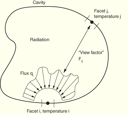
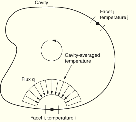
The two differing cavity radiation approaches are depicted in Figure 37.1.1–1 and Figure 37.1.1–2. The fully implicit method resolves the angular variation of the flux into each facet resulting from the different temperatures on the surface, the different emissivities, and the different geometric viewfactors. The approximate method uses a model of the flux that averages the spatially dependent contributions into a single term for the flux into each facet.
The approximate cavity radiation feature uses a simplified numerical model, based on specific physical and geometric assumptions:
the viewfactors between a given facet and all others are assumed to be equal;
blocking effects between facets are ignored;
emissivity is taken as constant over the entire surface; and
reflection effects between facets are ignored.
![]()
is the emissivity of facet ![]() ;
;
![]()
is the Stefan-Boltzmann constant;
![]()
is the geometrical viewfactor matrix;
![]()
are the temperatures of facets ![]() ; and
; and
![]()
is the absolute zero on the temperature scale used.

![]()
![]()
The averaged temperature is computed at the beginning of each increment and held constant over the increment. Therefore, the approximate method has some dependency on increment size and you need to ensure that the increment size you use is appropriate for your model. If you see large changes in temperature in the cavity over an increment, you may need to reduce the increment size.
When you define the model for an approximate cavity radiation problem, you must define the cavity as a single surface: only facets that are a part of a single surface will interact. The physical properties must also be defined (see “Defining the Stefan-Boltzmann constant and value of absolute zero”).
In an approximate cavity radiation analysis, the interacting radiating flux is specified using a surface radiation definition. You must designate that the surface-averaged interaction is to be used, and you must assign the emissivity of the surface.
| Input File Usage: | Use the following option to define approximate cavity radiation interaction on a surface: |
*SRADIATE surface name, AVG, , |
| Abaqus/CAE Usage: | Interaction module: Create Interaction: Surface radiation: select the surface region: Radiation type: Cavity approximation (3D only), Emissivity: |
Thermal-stress analysis can include approximate cavity radiation effects.
Emissivity, ![]() , is a dimensionless quantity with a value that is greater than or equal to zero and less than or equal to one. A value of
, is a dimensionless quantity with a value that is greater than or equal to zero and less than or equal to one. A value of ![]() corresponds to all radiation being reflected by the surface and, in this approximation, implies that the radiation flux is zero. A value of
corresponds to all radiation being reflected by the surface and, in this approximation, implies that the radiation flux is zero. A value of ![]() corresponds to black body radiation, where all radiation is absorbed by the surface. In the approximate cavity radiation method, the emissivity of a surface is assumed to be constant with respect to temperature and other predefined field variables.
corresponds to black body radiation, where all radiation is absorbed by the surface. In the approximate cavity radiation method, the emissivity of a surface is assumed to be constant with respect to temperature and other predefined field variables.
When using the approximate cavity radiation interaction approach, the radiation interaction uses the same symmetry as the model itself: no special cavity symmetry definitions apply.
In the approximate cavity radiation interaction approach, only the facets of the specified surface interact; there is no interaction with an ambient void. However, you can model an open cavity by defining an artificial enclosure with a boundary condition set to the reference temperature of the external medium. This ambient temperature value is converted to an absolute temperature scale based on the definition of absolute zero. The artificial enclosure should be created in the same manner as any other part in Abaqus.
To switch approximate cavity radiation effects on and off during the analysis, you can use a new surface radiation definition to switch the radiation on and off in any particular surface during one or more steps of the analysis.
| Abaqus/CAE Usage: | To deactivate radiation in a step: |
Interaction module: interaction manager: select a propagated interaction, Deactivate To activate radiation in a step, you must select the first step in which it was inactivated: Interaction module: interaction manager: select an interaction in the first step where it is inactive, Activate |
The fully implicit cavity radiation equations are not symmetric; therefore, the nonsymmetric matrix storage and solution scheme is invoked automatically in models that include cavity radiation (see “Cavity radiation,” Section 2.11.4 of the Abaqus Theory Manual, and “Procedures: overview,” Section 6.1.1). Each cavity defines an unsymmetric element matrix that couples the temperature degree of freedom of every node on every surface in the cavity. These matrices are typically updated a number of times during the analysis (due to temperature-dependent emissivity or moving surfaces in the cavity). Therefore, large cavity radiation problems may be computationally expensive. Moreover, there is a software limit of 16000 degrees of freedom that no element in Abaqus/Standard may exceed; this means that no single cavity definition in a model may have more than 16000 nodes.
Since fully implicit cavity radiation effects are calculated only in heat transfer and coupled thermal-electrical procedures, the only kind of thermal-stress analysis that can include these effects is sequentially coupled thermal-stress analysis (see “Sequentially coupled thermal-stress analysis,” Section 6.5.3).
When you define the model for a fully implicit cavity radiation problem, you must:
define all of the surfaces in the cavity (see “Defining surfaces”);
define the radiation properties of each surface (i.e., the emissivity) and the physical constants (see “Defining surface radiation properties”); and
construct cavities from the surfaces (see “Constructing a cavity for the fully implicit method”).
In the first step of a fully implicit cavity radiation analysis you must associate with each cavity a radiation viewfactor definition, which controls the calculation of viewfactors for the cavity. You then may:
define cavity symmetries, if any (see “Defining cavity symmetries”);
prescribe the motion of surfaces (see “Prescribing motion during a cavity radiation analysis”);
define boundary conditions such as temperature and forced convection (see “Boundary conditions”);
control the cavity radiation and viewfactor calculations in each step (the specifications from the previous step are used if they are not redefined in a step; see “Controlling viewfactor calculation during the analysis”);
request output of heat transfer variables to the data and results files (see “Requesting surface variable output”); and
request output of the radiation viewfactor matrices (see “Writing the viewfactor matrices to the results file”).
Cavities are defined in Abaqus/Standard as collections of surfaces, which are composed of facets. In axisymmetric and two-dimensional cases a facet is a side of an element; in three-dimensional cases a facet is a face of a solid element or a surface of a shell element. Rigid surfaces cannot be used in cavity radiation problems.
Surfaces are defined as described in “Defining element-based surfaces,” Section 2.3.2. You may associate each surface with a surface property definition as part of the surface option, or you may associate surfaces with surface properties as part of the cavity definition option. The surface properties are defined as described below.
| Input File Usage: | Use the following option to define a surface with a surface property for use in a cavity radiation analysis: |
*SURFACE, TYPE=ELEMENT, NAME=surface_name, PROPERTY=property_name Use the following option to define a surface for use in a cavity radiation analysis in which surface properties are defined as part of the cavity definition: *SURFACE, TYPE=ELEMENT, NAME=surface_name |
| Abaqus/CAE Usage: | Interaction module: Create Interaction: Cavity radiation: select the initial surface region |
Surfaces that are associated with fully implicit cavity radiation are subject to the following restrictions in addition to the general surface definition restrictions outlined in “Defining element-based surfaces,” Section 2.3.2:
Surfaces cannot overlap because of the ambiguity that would result in the associated property definitions and in the blocking specification.
A surface can be used only in one cavity definition (the same surface cannot appear in two different cavities).
Surfaces should not be too close, relative to their characteristic sizes. Viewfactor calculations in this case may involve ill-conditioned or non-positive-definite matrices. Modifications to the model or the definition of heat radiation (see “Thermal contact properties,” Section 33.2.1) will help avoid this problem.
Facets that are not distant to each other (on the order of a typical facet length) should be of similar sizes. Otherwise, the approximations used during viewfactor calculations might result in viewfactors greater than one.
Cavity radiation problems are intrinsically nonlinear, due to the ![]() dependence of the flux. Further nonlinearity can be introduced by describing the emissivity,
dependence of the flux. Further nonlinearity can be introduced by describing the emissivity, ![]() , as a function of temperature. Emissivity is used in the cavity radiation formulation, where we write the radiation flux per unit area into a cavity facet as
, as a function of temperature. Emissivity is used in the cavity radiation formulation, where we write the radiation flux per unit area into a cavity facet as
![]()
are the emissivities of facets ![]() ;
;
![]()
is the Stefan-Boltzmann constant;
![]()
is the geometrical viewfactor matrix;
![]()
is the reflection matrix, ![]() ;
;
![]()
are the temperatures of facets ![]() ; and
; and
![]()
is the absolute zero on the temperature scale used.
In the fully implicit method, the radiation flux for each facet is calculated based on the average of the nodal temperatures on that facet (see “Cavity radiation,” Section 2.11.4 of the Abaqus Theory Manual). This value of radiation flux is then distributed to each node in proportion to its area. Consequently, the mesh must be sufficiently fine that temperature differences across elements are small. Otherwise, computed fluxes at nodes with temperatures above the facet average will be excessively low, and the fluxes at nodes with below-average temperatures will be too high. This tends to induce a spatially oscillatory solution. This effect can be eliminated by reducing element size in the vicinity of high temperature gradients.
In the fully implicit cavity radiation method, there is more flexibility in defining the emissivity. You can define the emissivity, ![]() , of a surface as a function of temperature and other predefined field variables. Emissivity is a dimensionless quantity with a value that is greater than or equal to zero and less than or equal to one. A value of
, of a surface as a function of temperature and other predefined field variables. Emissivity is a dimensionless quantity with a value that is greater than or equal to zero and less than or equal to one. A value of ![]() corresponds to all radiation being reflected by the surface. A value of
corresponds to all radiation being reflected by the surface. A value of ![]() corresponds to black body radiation, where all radiation is absorbed by the surface. If all surfaces in a given cavity have
corresponds to black body radiation, where all radiation is absorbed by the surface. If all surfaces in a given cavity have ![]() , the analysis will be much more efficient if you specify that heat reflection should be ignored in the cavity radiation calculations for a particular step. By default, heat reflection is included.
, the analysis will be much more efficient if you specify that heat reflection should be ignored in the cavity radiation calculations for a particular step. By default, heat reflection is included.
You must assign a name to the surface property that defines the emissivity.
| Input File Usage: | Use both of the following options to define the emissivity of a surface: |
*SURFACE PROPERTY, NAME=property_name
*EMISSIVITY
The *EMISSIVITY option must appear directly after the *SURFACE PROPERTY option in the model definition section of the input file. If black body radiation is being defined ( *RADIATION VIEWFACTOR, REFLECTION=NO |
| Abaqus/CAE Usage: | Use the following input to define gray body radiation: |
Interaction module: Create Interaction Property: Cavity radiation:
enter the emissivity ( You can define the emissivity as a function of temperature and/or field variables. Use the following input to define black body radiation: Interaction module: Create Interaction: Cavity radiation: Use heat reflection: No |
In the fully implicit method, Abaqus/Standard evaluates the emissivity, ![]() , based on the temperature at the start of each increment and uses that emissivity value throughout the increment. When emissivity is a function of temperature or field variables, you can control the time incrementation for the heat transfer or coupled thermal-electrical step by specifying the maximum allowable emissivity change during an increment,
, based on the temperature at the start of each increment and uses that emissivity value throughout the increment. When emissivity is a function of temperature or field variables, you can control the time incrementation for the heat transfer or coupled thermal-electrical step by specifying the maximum allowable emissivity change during an increment, ![]() . If this tolerance is exceeded, Abaqus/Standard will cut back the increment size until the maximum change in emissivity is less than the specified value. If you do not specify a value for
. If this tolerance is exceeded, Abaqus/Standard will cut back the increment size until the maximum change in emissivity is less than the specified value. If you do not specify a value for ![]() , a default value of 0.1 is used.
, a default value of 0.1 is used.
| Input File Usage: | Use either of the following options: |
*HEAT TRANSFER, MXDEM= |
| Abaqus/CAE Usage: | Step module: Create Step: Heat transfer or Coupled thermal-electric:
Incrementation: Automatic: Max. allowable emissivity change per increment: |
You must define the Stefan-Boltzmann constant, ![]() , and the value of absolute zero,
, and the value of absolute zero, ![]() ; there are no default values for these constants.
; there are no default values for these constants.
| Input File Usage: | *PHYSICAL CONSTANTS, STEFAN BOLTZMANN= |
This option can appear anywhere in the model definition portion of the input file. |
| Abaqus/CAE Usage: | Any module: Model |
You construct cavities as collections of the surfaces defined as described above. Each surface can be used only in one cavity definition. Each cavity must have a unique name; this name is used to specify viewfactor calculations. The cavity name can also be used to request output.
By default, a cavity is assumed to consist of surfaces for which surface properties have already been defined. Instead, you may define surface properties as part of the cavity definition.
| Input File Usage: | Use the following option to construct a cavity: |
*CAVITY DEFINITION, NAME=cavity_name, SET PROPERTY
surface name, surface property name
By using the SET PROPERTY parameter, you define the surface properties used in the cavity, overriding any property defined as part of the surface option. |
| Abaqus/CAE Usage: | Interaction module: Create Interaction: Cavity radiation: select the surface region. Use the Properties table to add or edit surfaces and cavity radiation interaction properties (emissivity). |
By default, a cavity is assumed to be closed.
| Input File Usage: | Use the following option to construct a closed cavity: |
*CAVITY DEFINITION, NAME=cavity_name |
| Abaqus/CAE Usage: | Interaction module: Create Interaction: Cavity radiation: Definition: Closed |
You can specify an open cavity by defining the reference temperature of the external medium. This ambient temperature value is converted to an absolute temperature scale based on the definition of absolute zero. You can verify the degree of opening in the cavity by specifying a tolerance for the accuracy of the viewfactor calculations; radiation to the external medium will take place only if the deviation of the sum of the viewfactors from unity is more than this tolerance. See “Controlling the accuracy of viewfactor calculations” below for details.
| Input File Usage: | Use the following option to create an open cavity: |
*CAVITY DEFINITION, NAME=cavity_name, AMBIENT TEMP= |
| Abaqus/CAE Usage: | Interaction module: Create Interaction: Cavity radiation: Definition: Open, Ambient temperature: |
The open cavity definition allows for a cavity with a single opening into an ambient environment with a single, constant temperature value. If the cavity has multiple openings or the ambient temperature is not constant, you should model the surroundings differently.
You should close any cavity openings with elements, and prescribe the temperatures of the external media on these elements. Since the cavity is now closed, you should not specify an ambient temperature with the cavity definition. The temperature definition that you use for the closing elements provides the ambient temperature, and it allows you to specify different temperatures, including variable temperatures, at the cavity openings. The elements modeling the external media should not share nodes with the cavity elements (so that conduction will not take place between them). The surfaces defined by the external media elements should have an emissivity of 1.
Taking advantage of geometric symmetry can reduce computational model size and simulation time in the fully implicit method. Instead of modeling all of the parts or components in a symmetric assembly, you can model a smaller repeated component and take symmetry into account in the definition of the cavity radiation interaction. In Abaqus/Standard cavity definitions with defined symmetries take into account the radiation interactions between each cavity facet and between all of the facets in the cavity and all of its symmetric images. Abaqus/Standard does not check that the model created using cavity symmetries is physically realistic. You must check the input and results carefully to ensure that a valid model is created.
You must assign a name to each radiation symmetry definition for reference by a radiation viewfactor definition. The radiation viewfactor definition and corresponding radiation symmetry definition must appear in the same step.
Cyclic, periodic, and/or reflection symmetries can be defined as described below.
| Input File Usage: | Use all of the following options to define symmetry in a cavity radiation problem: |
*RADIATION VIEWFACTOR, SYMMETRY=symmetry_name *RADIATION SYMMETRY, NAME=symmetry_name *REFLECTION and/or *PERIODIC and/or *CYCLIC |
| Abaqus/CAE Usage: | Interaction module: Create Interaction: Cavity radiation: Symmetry: Reflection, Periodic, and/or Cyclic |
You define reflection symmetry to create a cavity that is composed of the user-defined cavity surface plus its reflected image through a line or plane. You must identify the dimensionality of the cavity when you define reflection symmetry.
You can define the cavity symmetry by reflecting the cavity surface through a line, as shown in Figure 37.1.1–3. This type of reflection can be used only with two-dimensional cavities.
| Input File Usage: | *REFLECTION, TYPE=LINE |
| Abaqus/CAE Usage: | Interaction module: Create Interaction: Cavity radiation: Symmetry: Reflection: select the symmetry line |
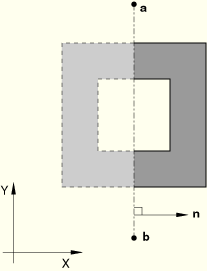
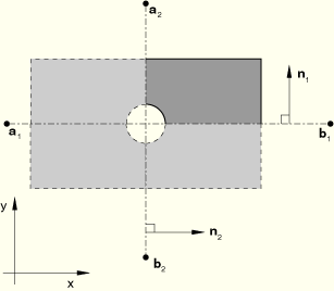
You can define the cavity symmetry by reflecting the cavity surface through a plane, as shown in Figure 37.1.1–4. This type of reflection can be used only with three-dimensional cavities.
| Input File Usage: | *REFLECTION, TYPE=PLANE |
| Abaqus/CAE Usage: | Interaction module: Create Interaction: Cavity radiation: Symmetry: Reflection: select the symmetry plane |
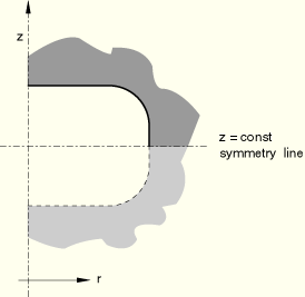
You can define the cavity symmetry by reflecting the cavity surface through a line of constant z-coordinate, as shown in Figure 37.1.1–5. This type of reflection can be used only with axisymmetric cavities.
| Input File Usage: | *REFLECTION, TYPE=ZCONST |
| Abaqus/CAE Usage: | Interaction module: Create Interaction: Cavity radiation: Symmetry: Reflection: enter the z-axis symmetry value for the line of symmetry |
You can define cavity symmetry by periodic repetition in a given direction. Physically, periodic symmetry is understood as an infinite number of repetitions of the same image at a periodic interval. Numerically, periodic symmetry has to be represented by a finite number of repetitions of the periodic image. You can define the number of repetitions used in the numerical calculation, n.
The periodic symmetry will result in a cavity composed of the user-defined cavity plus twice n similar images, since the periodic symmetry is assumed to apply in both the positive and negative directions. By default, n=2.
Although symmetries do not increase the size of the viewfactor matrix, they do make its calculation more expensive. Therefore, the number of repetitions should be minimized, but the value of n should be large enough that the viewfactor matrix is calculated accurately. Output variable VFTOT can be used to check the amount of closure implied by the symmetry. (See “Controlling the accuracy of viewfactor calculations” below.) Periodic symmetry for defining the cavity radiation viewfactor matrix does not impose symmetry conditions automatically in the heat transfer analysis. It may be necessary to impose appropriate constraints on the temperature and loading conditions at the nodes on the periodic symmetry planes to obtain a meaningful solution from the underlying heat transfer analysis.
You must identify the dimensionality of the cavity when you define periodic symmetry.
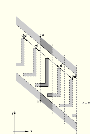
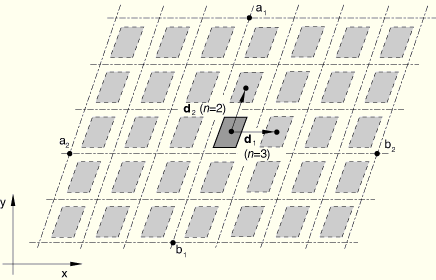
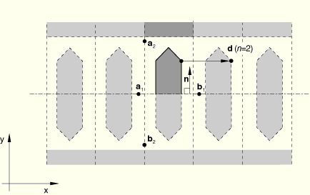
You can create a cavity that is composed of a series of similar images generated by repetition along a two-dimensional distance vector, as shown in Figure 37.1.1–6.
The repeated images are bounded by lines parallel to line ab. The distance vector must be defined so that it points away from line ab and into the domain of the model. This type of periodic symmetry can be used only with two-dimensional cavities.| Input File Usage: | *PERIODIC, TYPE=2D, NR=n |
| Abaqus/CAE Usage: | Interaction module: Create Interaction: Cavity radiation: Symmetry: Periodic: Number of periodic symmetries: n |
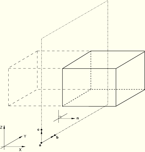
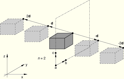
You can create a cavity that is composed of a series of similar images generated by repetition along a three-dimensional distance vector, as shown in Figure 37.1.1–7. The repeated images are bounded by planes that are parallel to plane abc. The distance vector must be defined so that it points away from plane abc and into the domain of the model. This type of periodic symmetry can be used only with three-dimensional cavities.
| Input File Usage: | *PERIODIC, TYPE=3D, NR=n |
| Abaqus/CAE Usage: | Interaction module: Create Interaction: Cavity radiation: Symmetry: Periodic: Number of periodic symmetries: n |
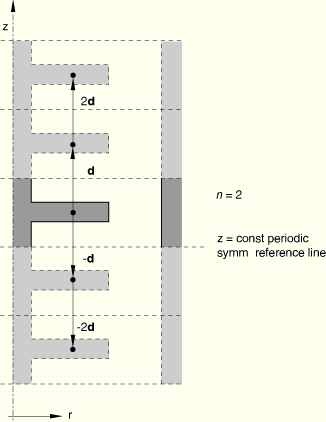
You can create a cavity that is composed of a series of similar images generated by repetition in the z-direction, as shown in Figure 37.1.1–8.
The repeated images are bounded by lines of constant z-coordinate. The z-distance vector must be defined so that it points away from the z-constant periodic symmetry reference line and into the domain of the model. This type of periodic symmetry can be used only with axisymmetric cavities.| Input File Usage: | *PERIODIC, TYPE=ZDIR, NR=n |
| Abaqus/CAE Usage: | Interaction module: Create Interaction: Cavity radiation: Symmetry: Periodic: Number of periodic symmetries: n |
You can define cavity symmetry by cyclic repetition of the user-defined cavity surface about a point or an axis. The cavity defined by cyclic repetition must cover 360°.
You must define the number of cyclically similar images that compose the cavity, n. The angle of rotation about a point or axis used to create cyclically similar images is equal to 360°/n.
You must identify the dimensionality of the cavity when you define cyclic symmetry.
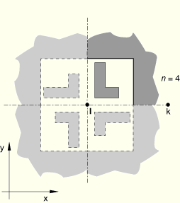
You can define the cavity symmetry by rotating the cavity about a point, l, as shown in Figure 37.1.1–9.
The cavity surface defined in the model must be bounded by the line lk and a line passing through l at an angle, measured counterclockwise when looking into the plane of the model, of 360°/n to lk. This type of cyclic symmetry can be used only for two-dimensional cavities.| Input File Usage: | *CYCLIC, TYPE=POINT, NC=n |
| Abaqus/CAE Usage: | Interaction module: Create Interaction: Cavity radiation: Symmetry: Cyclic: toggle on Use cyclic symmetric, Total number of sectors: n |
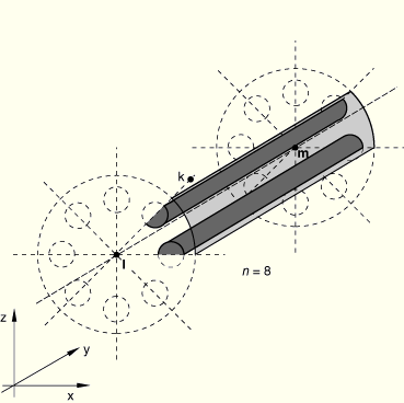
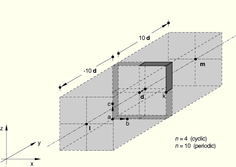
You can define the cavity symmetry by rotating the cavity about an axis, lm, as shown in Figure 37.1.1–10. The cavity surface defined in the model must be bounded by the plane lmk and a plane passing through the line lm at an angle, measured clockwise when looking from l to m, of 360°/n to lmk. Line lk must be normal to line lm. This type of cyclic symmetry can be used only for three-dimensional cavities.
| Input File Usage: | *CYCLIC, TYPE=AXIS, NC=n |
| Abaqus/CAE Usage: | Interaction module: Create Interaction: Cavity radiation: Symmetry: Cyclic: toggle on Use cyclic symmetric, Total number of sectors: n |
Reflection, periodic, and cyclic symmetries can be combined as shown in Table 37.1.1–1. Figure 37.1.1–11 through Figure 37.1.1–14 illustrate some possible symmetry combinations.
Table 37.1.1–1 Permissible number of symmetry definitions used in combination.
| Reflection | Periodic | Cyclic | 2-D | 3-D | Axi | Restrictions |
|---|---|---|---|---|---|---|
| 1 | 0 | 0 | • | • | • | |
| 2 | 0 | 0 | • | • | ||
| 3 | 0 | 0 | • | |||
| 0 | 1 | 0 | • | • | • | |
| 0 | 2 | 0 | • | • | ||
| 0 | 3 | 0 | • | |||
| 1 | 1 | 0 | • | • | ||
| 1 | 2 | 0 | • | |||
| 2 | 1 | 0 | • | |||
| 0 | 0 | 1 | • | • | ||
| 1 | 0 | 1 | • | |||
| 0 | 1 | 1 | • |
![]() ,
, ![]() ,
, ![]() ,
, ![]() are normals to lines or planes of reflection symmetry.
are normals to lines or planes of reflection symmetry.
![]() ,
, ![]() ,
, ![]() are distance vectors used to define periodic symmetry.
are distance vectors used to define periodic symmetry.
![]() is the direction of the axis of cyclic symmetry in three-dimensional cases.
is the direction of the axis of cyclic symmetry in three-dimensional cases.
In many cavity radiation problems such as simulations of manufacturing sequences, radiation viewfactors change because surfaces are moved during the analysis. You can specify surface motions during heat transfer or coupled thermal-electrical analysis.
The prescribed motions affect only the calculation of viewfactors (and, therefore, radiation fluxes) in heat transfer due to cavity radiation. They do not affect heat conduction, storage, or distributed flux contributions.
You can define both the translational and rotational components of the motion within a step independently. For example, you can prescribe the translational motion of a node set according to a certain amplitude function and then prescribe the rotational motion of the node set according to a different amplitude function. In each step, each component of motion can be specified only once for any particular node.
Motions can also be prescribed during steps in which the cavity radiation is turned off, as described below.
Translations, ![]() , are specified in terms of global x-, y-, and z-components unless a local coordinate system is defined at the nodes for which motion is specified; then translations are specified in terms of local x-, y-, and z-components (see “Transformed coordinate systems,” Section 2.1.5).
, are specified in terms of global x-, y-, and z-components unless a local coordinate system is defined at the nodes for which motion is specified; then translations are specified in terms of local x-, y-, and z-components (see “Transformed coordinate systems,” Section 2.1.5).
Translational displacements are always specified as total values of translational motion. This treatment of translations is consistent with that used for displacement boundary conditions (“Boundary conditions,” Section 30.3.1) in stress/displacement analyses. The default is to apply translational motion.
Translational velocities can also be specified. Translational velocities always refer to the current step; therefore, the rate of translational motion specified as a velocity is in effect only during the step for which it is defined. This behavior is different from velocity boundary conditions, where velocities stay in effect in subsequent steps if they are not redefined.
| Abaqus/CAE Usage: | Surface motion is not supported with cavity radiation in Abaqus/CAE. |
Displacements due to a rigid body rotation, ![]() , can be defined by specifying the magnitude of the rotation and the rotation axis. In three dimensions the rotation axis is defined by specifying two points,
, can be defined by specifying the magnitude of the rotation and the rotation axis. In three dimensions the rotation axis is defined by specifying two points, ![]() and
and ![]() , on the axis of rotation. In two dimensions the rotation axis is assumed to be normal to the plane of the model and is defined by specifying one point,
, on the axis of rotation. In two dimensions the rotation axis is assumed to be normal to the plane of the model and is defined by specifying one point, ![]() .
.
The coordinates of the points defining the axis of rotation must be defined in the configuration at the beginning of the step for which rigid body rotation is being defined.
Motion due to rigid body rotation during a step is specified as the amount of rotation that takes place during that step only. Therefore, the rigid body rotation specified during a step is local to that step; if no rigid body rotation is specified in the following step, no further rotation occurs.
The treatment of rigid body rotations is different from that of translations: rigid body rotations are specified incrementally from step to step while translations are specified as total values.
| Abaqus/CAE Usage: | Surface motion is not supported with cavity radiation in Abaqus/CAE. |
Prescribed rotational motions of more than ![]() radians or complex sequences of rotations about different directions in three-dimensional models are most simply defined by specifying rotational velocities, which allows the definition to be given in terms of the angular velocity instead of the total rotation. Abaqus/Standard calculates the increment of rotation as the average of the angular velocities at the beginning and end of each increment multiplied by the time increment. (See “Conventions,” Section 1.2.2.)
radians or complex sequences of rotations about different directions in three-dimensional models are most simply defined by specifying rotational velocities, which allows the definition to be given in terms of the angular velocity instead of the total rotation. Abaqus/Standard calculates the increment of rotation as the average of the angular velocities at the beginning and end of each increment multiplied by the time increment. (See “Conventions,” Section 1.2.2.)
For example, if a rotation of ![]() about the z-axis is required, with no rotation about the x- and y-axes, and assuming a step time of 1.0, specify a constant angular velocity of
about the z-axis is required, with no rotation about the x- and y-axes, and assuming a step time of 1.0, specify a constant angular velocity of ![]() as follows:
as follows:
*MOTION, TYPE=VELOCITY, ROTATION
 node (node set), 18.84955592, 0., 0., 0., 0., 0., 1.
The angular velocity will be constant since the default variation for motions prescribed using a predefined velocity field in a heat transfer or coupled thermal-electrical step (both steady-state and transient) is a step function (see “Procedures: overview,” Section 6.1.1). An amplitude reference could be used to specify other variations of the angular velocity.
If, in the next step, the same node (or node set) should have an additional rotation of ![]() radians about the global x-axis, assuming again a step time of 1.0, prescribe a constant angular velocity as follows:
radians about the global x-axis, assuming again a step time of 1.0, prescribe a constant angular velocity as follows:
*MOTION, TYPE=VELOCITY, ROTATION
 node (node set), 1.570796327, 0., 0., 0., 1., 0., 0.
Motions involving two or more simultaneous rigid body rotations about different axes cannot be specified directly. An example of simultaneous rigid body rotations is a satellite rotating about its own axis while orbiting the earth. Such complex motions can be defined with user subroutine UMOTION. This subroutine allows specification of the time variation of the magnitude of the translational components of the motion (degrees of freedom 1–3) at each node.
If you specify the magnitude of the translation as part of the prescribed motion definition, it will be modified by the amplitude curve (if any) and passed into subroutine UMOTION, where it can be redefined.
When user subroutine UMOTION is used to define the motion of a certain node set in a step, only one prescribed motion can be defined in that step for that node set. The complete motion of all nodes in the node set during the step must be defined in the user subroutine.
| Input File Usage: | *MOTION, USER |
| Abaqus/CAE Usage: | Surface motion is not supported with cavity radiation in Abaqus/CAE. |
Whenever simultaneous translational and rotational motion is specified, the total motion of a node during step k is defined as
In these cases the translation is applied first and the rotation is then assumed to be about the translated (material) axis. In other words, the displacement ![]() due to rigid body rotation during step i is computed as the rotation about an axis defined by points
due to rigid body rotation during step i is computed as the rotation about an axis defined by points ![]() and
and ![]() where
where
![]()
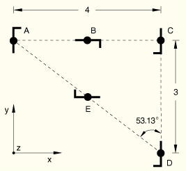
As an example, consider a three-dimensional problem with x–y planar motion as shown in Figure 37.1.1–15.
The centroid of the object of interest is initially located at ![]() . In the first step the object is translated 4 length units in the x-direction while at the same time it rotates clockwise 180° (
. In the first step the object is translated 4 length units in the x-direction while at the same time it rotates clockwise 180° (![]() radians) about the z-axis at constant angular velocity. This motion moves the object from position A to position C in Figure 37.1.1–15. Halfway through this motion, at position B, the displacements due to the rigid body rotation are calculated by applying the translation to the z-axis (the axis of rotation) and then applying a 90° rotation about this translated axis.
radians) about the z-axis at constant angular velocity. This motion moves the object from position A to position C in Figure 37.1.1–15. Halfway through this motion, at position B, the displacements due to the rigid body rotation are calculated by applying the translation to the z-axis (the axis of rotation) and then applying a 90° rotation about this translated axis.
In the second step the object is translated –3 length units in the y-direction only. This motion places the object at position D with no additional rotation. Finally, in the third step the object is simultaneously translated 5 length units at an angle of 53.13° to the y-direction and rotated clockwise, again at constant angular velocity, through 180° about the z-axis. This motion returns the object to its original position.
Assuming that each step time is 1.0, the input required for the above motion sequence is as follows:
First step:
*MOTION
 node set, 1, 1, 4.
*MOTION, ROTATION, TYPE=VELOCITY
 node set, 3.14159265, 0., 3., 0., 0., 3., -1.
Second step:
*MOTION
 node set, 2, 2, -3.
Third step:
*MOTION
 node set, 1, 2, 0.
*MOTION, ROTATION, TYPE=VELOCITY
 node set, 3.14159265, 4., 0., 0., 4., 0., -1.
For any prescribed motion you can refer to an amplitude curve that gives the time variation of the motion throughout a step (see “Amplitude curves,” Section 30.1.2).
| Input File Usage: | Use both of the following options: |
*AMPLITUDE, NAME=amplitude *MOTION, AMPLITUDE=amplitude |
| Abaqus/CAE Usage: | Surface motion is not supported with cavity radiation in Abaqus/CAE. |
You can control how viewfactors are recalculated during a step as a result of prescribed motion by specifying a value for the maximum allowable motion, max, for a particular node set. Viewfactor recalculation is triggered if a displacement component at any node in the specified node set exceeds the specified value for max.
You must respecify the value of max and the node set in every step where recalculation is required; the values do not remain in effect for subsequent steps.
Viewfactor recalculation can be expensive; use discretion when choosing a value for max.
| Input File Usage: | *RADIATION VIEWFACTOR, MDISP=max, NSET=nset |
The max and nset values must always be specified together. |
| Abaqus/CAE Usage: | Viewfactor recalculation due to motion is not supported with cavity radiation in Abaqus/CAE. |
The cavity radiation capability can be used in applications such as the simulation of manufacturing sequences where radiation viewfactors change during the simulation. Therefore, radiation viewfactor definitions provide significant flexibility for the control of viewfactor calculations during a step.
Multiple radiation viewfactor definitions can be specified within a step definition if different types of radiation and viewfactor calculations are required for different cavities. Different types of viewfactor calculations can be specified for the same cavity in different steps of the analysis.
By default, viewfactors are calculated at the beginning of the first step that includes a radiation viewfactor definition. Viewfactors are recalculated at the beginning of a subsequent step only if the viewfactor definition changes in that step; for example, if different surface blocking checks are specified for the same cavity. In a restart analysis Abaqus/Standard reads the radiation viewfactors from the user-specified restart step and increment and recalculates the viewfactors only if the viewfactor definitions have changed.
You can specify the name of the cavity for which radiation viewfactor control is being specified. If you do not specify a cavity name, the radiation viewfactor definition applies to all cavities in the model.
| Input File Usage: | *RADIATION VIEWFACTOR, CAVITY=cavity_name |
| Abaqus/CAE Usage: | Radiation viewfactors are defined separately for each cavity radiation interaction and apply to all steps in which that interaction is active. |
There are practical situations in which it may be useful to switch cavity radiation effects on and off during the analysis. For example, radiation may be taking place in a cavity that is then filled with a fluid so that radiation is no longer significant; later in the analysis, radiation may resume when the fluid is drained from the cavity. In such cases you can use a radiation viewfactor definition to switch the radiation on and off in any particular cavity during one or more steps of the analysis.
When cavity radiation is switched on after having been switched off, Abaqus/Standard will use the last viewfactors calculated in the last step in which cavity radiation was active. However, if motion is prescribed during the time that the cavity radiation is switched off and one of the displacement components of a node in the specified node set exceeds the value for the maximum allowable motion, max, specified in the step during which cavity radiation is switched off, the viewfactors will be recalculated at the beginning of the step in which the cavity radiation is switched back on.
| Input File Usage: | Use the following option to turn viewfactor calculation off for a step: |
*RADIATION VIEWFACTOR, OFF Use one of the following options to turn viewfactor calculation back on in a subsequent step: *RADIATION VIEWFACTOR *RADIATION VIEWFACTOR, MDISP=max, NSET=nset |
| Abaqus/CAE Usage: | Radiation viewfactors cannot be turned off or on for a selected step. You can use the following options to turn a cavity radiation interaction off or on: |
Interaction module: Interaction Manager: select a step and a cavity radiation interaction, Activate or Deactivate |
You can provide a tolerance on the accuracy of the viewfactor calculation. In a closed cavity the sum of the viewfactors for each cavity facet should be one. Abaqus/Standard compares the value of the specified tolerance to the deviation of the average sum from unity (the average sum is computed by summing the sums of the viewfactors over all the facets and dividing it by the number of facets). If the tolerance is violated for a closed cavity, the analysis is terminated. The default viewfactor tolerance is 0.05. Failure to meet this criterion may indicate a need for mesh refinement.
| Input File Usage: | *RADIATION VIEWFACTOR, VTOL=tolerance |
| Abaqus/CAE Usage: | Interaction module: Create interaction: Cavity radiation: Viewfactors: Accuracy tolerance: tolerance |
The viewfactor calculations account for the closure of a cavity implied by any cavity symmetries. For cavities without periodic or cyclic symmetries the viewfactors are calculated exactly for two-dimensional geometries, but approximations are made for axisymmetric and three-dimensional geometries. These approximations become less accurate as the distance between surfaces decreases. Define heat radiation to model closely spaced surfaces (see “Thermal contact properties,” Section 33.2.1).
If the sum of the viewfactors for facets in an open cavity (defined by specifying a value for the ambient temperature) deviates from unity by more than the specified viewfactor tolerance, radiation to the ambience will take place. In nearly closed cavities this deviation may be small. If the tolerance is not violated, radiation to the external medium is not included even though the cavity is defined to be open; a warning message is issued to this effect. You can loosen the viewfactor tolerance to include such radiation.
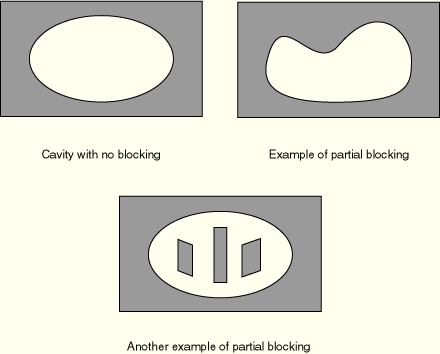
Heat is transferred between surfaces that have unobstructed direct views of each other (see Figure 37.1.1–16); “blocking” may occur in geometrically complex cavities.
Surface blocking checks may be computationally expensive in cavities with many surfaces; therefore, significant computational time may be saved by specifying which surfaces are potential blocking surfaces, as described below.
Viewfactor calculations with blocking surfaces are especially sensitive to mesh refinement. If a mesh is too coarse, the viewfactors may not add up to one (in a closed cavity). To obtain accurate results, the mesh should be refined until the viewfactors can be summed accurately.
By default, Abaqus/Standard will check for blocking of every surface with itself and all other surfaces.
| Input File Usage: | *RADIATION VIEWFACTOR, BLOCKING=ALL |
| Abaqus/CAE Usage: | Interaction module: Create interaction: Cavity radiation: Properties: Blocking surface checks: All |
You can specify a list of the potential blocking surfaces in the cavity.
| Input File Usage: | *RADIATION VIEWFACTOR, BLOCKING=PARTIAL |
| Abaqus/CAE Usage: | Interaction module: Create interaction: Cavity radiation: Properties: Blocking surface checks: Partial |
You can indicate that there are no blocking surfaces in the cavity; in this case Abaqus omits all checks for blocking.
| Input File Usage: | *RADIATION VIEWFACTOR, BLOCKING=NO |
| Abaqus/CAE Usage: | Interaction module: Create interaction: Cavity radiation: Properties: Blocking surface checks: None |
In cases where there are many surfaces in the cavity, surfaces separated by more than a certain distance may not be able to “see” each other for the purposes of radiation because of blocking by other surfaces. You can specify the distance beyond which viewfactors need not be calculated, which reduces the computational effort required for the viewfactor calculations.
| Input File Usage: | *RADIATION VIEWFACTOR, RANGE=distance |
| Abaqus/CAE Usage: | Interaction module: Create interaction: Cavity radiation: Viewfactors: toggle on Specify blocking range: distance |
The cavity radiation heat transfer between facets of a surface in Abaqus is modeled using a full, unsymmetric matrix defining interactions between each node and all others in the cavity. For surfaces with large numbers of nodes this matrix may be large, resulting in memory requirements that are significantly larger than those for the finite element portion of the analysis without the cavity radiation interaction.
To minimize memory requirements and computational cost for cavity radiation heat transfer analysis, the cavity can be defined using a coarser mesh of heat transfer shell elements having a single degree of freedom per node. The overlaid element should have minimal heat capacity and conduction, and it should be used for the definition of the cavity in place of the physical, multiple-degree-of-freedom shell. The overlaid element should be used to define the master surface in a tied coupling constraint (“Mesh tie constraints,” Section 31.3.1); the multiple-degree-of-freedom, physical, heat transfer shell element forms the slave surface.
If the approximate, diagonally implicit method is appropriate for the problem of interest, using this method will reduce computational burdens substantially.
By default, the initial temperature of all nodes is zero. You can specify nonzero initial temperatures in a cavity radiation analysis; see “Defining initial temperatures” in “Initial conditions,” Section 30.2.1.
In a heat transfer analysis involving forced convection through the mesh, you can define nonzero initial mass flow rates at the nodes of the forced convection/diffusion heat transfer elements in the model (see “Uncoupled heat transfer analysis,” Section 6.5.2).
You can specify boundary conditions to prescribe temperatures (degree of freedom 11) at the nodes (see “Boundary conditions,” Section 30.3.1). Shell elements have additional temperature degrees of freedom 12, 13, etc. through the thickness (see “Conventions,” Section 1.2.2). Boundary conditions can be specified as functions of time by referring to amplitude curves (“Amplitude curves,” Section 30.1.2).
For purely diffusive elements, a boundary without any prescribed boundary conditions (natural boundary condition) corresponds to an insulated surface. For forced convection/diffusion elements, only the flux associated with conduction is zero; energy is free to convect across an unloaded surface. This natural boundary condition correctly models areas where fluid is crossing a surface (as, for example, at the upstream and downstream boundaries of the mesh) and prevents spurious reflections of energy back into the mesh.
The following types of loading can be prescribed in addition to the fully implicit cavity radiation, as described in “Thermal loads,” Section 30.4.4:
Concentrated heat fluxes
Body fluxes and distributed surface fluxes
Convective film conditions and radiation conditions
You cannot specify temperatures as field variables in heat transfer or coupled thermal-electrical analyses. Boundary conditions should be used instead, as described above.
You can specify values of other user-defined field variables during the analysis. These values will affect field-variable-dependent material properties, if any. See “Predefined fields,” Section 30.6.1.
You must define the radiation properties of the surfaces as described above in “Defining surface radiation properties.” Other thermal properties such as conductivity, density, specific heat, and latent heat are defined as in uncoupled heat transfer analysis—see “Uncoupled heat transfer analysis,” Section 6.5.2, and “Thermal properties: overview,” Section 23.2.1.
You can specify internal heat generation—see “Internal heat generation” in “Uncoupled heat transfer analysis,” Section 6.5.2.
Thermal expansion coefficients are not meaningful in cavity radiation heat transfer analysis since deformation of the structure is not considered.
Any of the heat transfer or coupled thermal-electrical elements in Abaqus/Standard can be used in a cavity radiation analysis, including forced convection/diffusion heat transfer elements (see “Choosing the appropriate element for an analysis type,” Section 24.1.3; “Uncoupled heat transfer analysis,” Section 6.5.2; and “Coupled thermal-electrical analysis,” Section 6.6.2). Coupled temperature-displacement elements cannot be used in a cavity radiation analysis.
In addition to the elements that you define, Abaqus/Standard uses internal elements that are generated automatically from your definition of radiation cavities.
The following output variables are available for fully implicit cavity radiation:
RADFL | Radiation flux per unit area. This variable does include heat flux to ambient in an open cavity. |
RADFLA | Radiation flux over a facet. |
RADTL | Time integrated radiation per unit area. |
RADTLA | Time integrated radiation over a facet. |
VFTOT | Total viewfactor for a facet (sum of the viewfactor values in the row of the viewfactor matrix corresponding to the facet). |
FTEMP | Facet temperature. |
You can write the viewfactor matrices for fully implicit cavity radiation interactions in heat transfer or coupled thermal-electrical analyses to the results (.fil) file. The entire radiation viewfactor matrix is written for each cavity radiation element in the specified cavity.
You can control the frequency of viewfactor matrix output by specifying the required output frequency in increments. The default output frequency is 1. Specify an output frequency of 0 to suppress output. The output will always be written at the last increment of each step unless you specify an output frequency of 0.
The record formats for the results file are described in “Results file output format,” Section 5.1.2. The file can be written in binary or ASCII format (see “Controlling the format of the results file in Abaqus/Standard” in “Output,” Section 4.1.1).
| Input File Usage: | *VIEWFACTOR OUTPUT, CAVITY=cavity_name, FREQUENCY=n |
| Abaqus/CAE Usage: | Viewfactor output is not supported in Abaqus/CAE. |
For the fully implicit cavity radiation interaction, you can request cavity-, element-, or surface-based radiation output such as radiation fluxes, viewfactor totals for a facet, and facet temperatures to the data, results, and/or output database files. The output requests can be repeated as often as necessary to request output for different variables, different cavities, different surfaces, different element sets, etc. The surface variables that can be requested are listed above.
You can specify the particular cavity, element set, or surface for which output is being requested. If you do not specify a cavity, element set, or surface, output will be provided for all cavities in the model. The same cavity, element set, or surface can appear in several radiation output requests.
By default, no cavity radiation data output will be provided. If you define a radiation output request without specifying the desired output variables, all six cavity radiation surface variables will be output.
You can control the frequency of radiation output by specifying the required output frequency in increments. The default output frequency is 1. Specify an output frequency of 0 to suppress output. The output will always be written at the last increment of each step unless you specify an output frequency of 0.
| Input File Usage: | Use one of the following options to obtain output in the data file: |
*RADIATION PRINT, CAVITY=cavity_name, FREQUENCY=n
*RADIATION PRINT, ELSET=element_set, FREQUENCY=n
*RADIATION PRINT, SURFACE=surface_name, FREQUENCY=n
Use one of the following options to obtain output in the results file: *RADIATION FILE, CAVITY=cavity_name, FREQUENCY=n *RADIATION FILE, ELSET=element_set, FREQUENCY=n *RADIATION FILE, SURFACE=surface_name, FREQUENCY=n Use the first option and one of the subsequent options to obtain output in the output database: *OUTPUT, FREQUENCY=n *RADIATION OUTPUT, CAVITY=cavity_name *RADIATION OUTPUT, ELSET=element_set *RADIATION OUTPUT, SURFACE=surface_name |
| Abaqus/CAE Usage: | Cavity radiation output to the data file and the results file are not supported in Abaqus/CAE. |
Use the following options to obtain output in the output database: Step module: history output request editor: Thermal: select the output variables |
The output tables generated by a radiation output request to the data file are organized on a surface-by-surface basis. The rows that will appear in a particular table are defined by choosing a cavity, surface, or element set: each row of a table corresponds to an individual element face that is part of the cavity, surface, or element set chosen. If all of the variables in a row of a table are zero, the row is not printed.
The first column of each table is the element number, and the second column is the element face identifier. You choose the variables to appear in the remaining columns. There is no limit to the number of tables that can be defined.
As an example, consider a heat transfer model containing a cavity named CAV1, which, in turn, is composed of surfaces SURF1 and SURF2. If you request output of radiation flux (RADFL) and facet temperature (FTEMP) to the data file for this model, two tables will appear in the data file. One table will contain RADFL and FTEMP output for all element faces composing surface SURF1, and the other table will contain the same output variables for all element faces making up surface SURF2.
By default, Abaqus/Standard writes a summary of the maximum and minimum values in each column of the table. You can choose to suppress this summary. In addition, you can choose to print the total of each column in the table, which is useful, for example, to sum radiation fluxes over all facets composing a radiation surface. By default, these totals are not printed.
| Input File Usage: | Use the following option to control output of the summary information to the data file: |
*RADIATION PRINT, SUMMARY=YES or NO Use the following option to control output of the totals to the data file: *RADIATION PRINT, TOTALS=YES or NO |
| Abaqus/CAE Usage: | Cavity radiation output to the data file is not supported in Abaqus/CAE. |
The following template shows the options required for a transient, fully implicit cavity radiation analysis of a closed two-dimensional symmetric cavity. All surfaces within the cavity topcav have the same emissivity. The surface surf2 moves (translation only) during the analysis. In the second step surface surf2 stops moving, cavity radiation is turned off, all thermal loads except the surface convection are removed, and a steady-state heat transfer analysis is conducted to determine the final temperature of the system.
*HEADING … *PHYSICAL CONSTANTS, ABSOLUTE ZERO=, STEFAN BOLTZMANN=
*SURFACE, NAME=surf1, PROPERTY=surfp elset1, S1 elset2, S2 *SURFACE, NAME=surf2, PROPERTY=surfp elset3, *SURFACE PROPERTY, NAME=surfp *EMISSIVITY Data lines to define the emissivity of the surfaces in the model *CAVITY DEFINITION, NAME=topcav surf1, surf2 *INITIAL CONDITIONS, TYPE=TEMPERATURE Data lines to prescribe initial temperatures at the nodes *AMPLITUDE, NAME=motion Data lines to define amplitude curve to be used for motion of surface surf2 *AMPLITUDE, NAME=film Data lines to define amplitude curve to be used for the convection film coefficient, h ************* ** Step 1 ************* *STEP *HEAT TRANSFER, MXDEM=
, DELTMX=
Data line to define incrementation *RADIATION VIEWFACTOR, CAVITY=topcav, VTOL=tol, SYMMETRY=outer, NSET=nset, MDISP=max *RADIATION SYMMETRY, NAME=outer *REFLECTION, TYPE=LINE Data line to define line of symmetry *MOTION, TRANSLATION, TYPE=DISPLACEMENT, AMPLITUDE=motion Data line to define motion of nodes on surface surf2 *CFLUX and/or *DFLUX Data lines to define concentrated and/or distributed fluxes *BOUNDARY Data lines to prescribe temperatures at selected nodes *FILM, FILM AMPLITUDE=film Data lines to define surface convection ** *RADIATION PRINT, CAVITY=topcav, SUMMARY=YES, TOTALS=YES Data lines requesting cavity radiation surface variable output *RADIATION FILE, CAVITY=topcav, FREQUENCY=4 Data lines requesting cavity radiation surface variable output *NODE PRINT Data lines requesting nodal output such as temperatures*EL PRINT Data lines requesting element output such as heat flux *END STEP ************* ** Step 2 ************* *STEP *HEAT TRANSFER, STEADY STATE Data line to define incrementation *RADIATION VIEWFACTOR, OFF *CFLUX, OP=NEW *DFLUX, OP=NEW *END STEP