Product: Abaqus/Standard
This example, taken from Collingwood et al. (1985), is intended to verify the coding of the time domain linear viscoelastic material model.
The problem is a rod of length of 254 mm (10 in) and diameter of 25.4 mm (1 in). The rod is fixed in the axial direction on one end and a constant axial load of 0.689 MPa (100 psi) is applied suddenly to the other end. The rod is modeled using one quadratic, axisymmetric, hybrid continuum element (CAX8H).
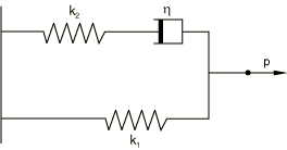
The linear viscoelastic material model used in this example can be represented by a combination of linear springs and a dashpot, as shown in Figure 3.1.11. The extensional relaxation function is
![]()
Short-term material properties are specified using the *ELASTIC option (“Linear elastic behavior,” Section 21.2.1 of the Abaqus Analysis User's Manual), which requires the instantaneous Young's modulus, ![]() , and Poisson's ratio,
, and Poisson's ratio, ![]() . The time-dependent behavior is specified using the *VISCOELASTIC option, in which the shear relaxation modulus and the bulk modulus are defined by a Prony series (see “Time domain viscoelasticity,” Section 21.7.1 of the Abaqus Analysis User's Manual). For the Abaqus analysis of this problem, it is assumed that no volumetric relaxation occurs.
. The time-dependent behavior is specified using the *VISCOELASTIC option, in which the shear relaxation modulus and the bulk modulus are defined by a Prony series (see “Time domain viscoelasticity,” Section 21.7.1 of the Abaqus Analysis User's Manual). For the Abaqus analysis of this problem, it is assumed that no volumetric relaxation occurs.
![]() is immediately available as
is immediately available as ![]() 68.9 MPa (10000 psi), and
68.9 MPa (10000 psi), and ![]() is
is
![]()
![]()
![]()
![]()
The shear relaxation time, ![]() , is obtained by writing the rate of change of the shear modulus in terms of the rate of change of the extensional modulus at time
, is obtained by writing the rate of change of the shear modulus in terms of the rate of change of the extensional modulus at time ![]() 0:
0:
![]()
![]()
The same problem is also treated as a large-strain example. The relaxation behavior is defined in the same way, but the short-term elastic properties are given with the *HYPERELASTIC option. The polynomial formulation with ![]() 1 is used, and the constants are
1 is used, and the constants are ![]() 6.89 MPa (1000 psi),
6.89 MPa (1000 psi), ![]() 4.59 MPa (666.67 psi), and
4.59 MPa (666.67 psi), and ![]() 1.378 × 10⁷ MPa1 (0.00002 psi1). These constants are such that the initial Young's modulus and initial Poisson's ratio are equal to
1.378 × 10⁷ MPa1 (0.00002 psi1). These constants are such that the initial Young's modulus and initial Poisson's ratio are equal to ![]() and
and ![]() , respectively, and produce a close fit to a linear material. (See “Hyperelastic behavior of rubberlike materials,” Section 21.5.1 of the Abaqus Analysis User's Manual, for further discussion of the choice of constants when
, respectively, and produce a close fit to a linear material. (See “Hyperelastic behavior of rubberlike materials,” Section 21.5.1 of the Abaqus Analysis User's Manual, for further discussion of the choice of constants when ![]() 1.)
1.)
A distributed load of 0.689 MPa (100 psi) is applied instantaneously and held constant throughout the analysis. To model this, we use the *VISCO procedure (“Quasi-static analysis,” Section 6.2.5 of the Abaqus Analysis User's Manual) in two steps. The load is applied in the first step, which has a time period of 0.001 seconds, so that the instantaneous (glassy) behavior dominates. Since this step uses only one increment, CETOL is not specified on the *VISCO option. The second step has a time period of 50 seconds, during which the load is held constant and the rod is allowed to relax toward its long-term behavior. Automatic time incrementation is chosen by giving a value for CETOL, the maximum difference in the creep strain increment over a time increment. CETOL is selected so that its value is of the same order of magnitude as the maximum elastic strain. Therefore, for this example CETOL is set to 5 × 10³. The *SECTION FILE option is used to output the total force and the total moment on the loaded face of the model.
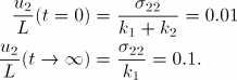
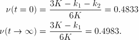
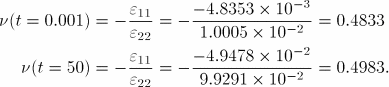
The instantaneous and long-term behaviors provide a check on the Abaqus results. The instantaneous and long-term axial displacements of the rod tip can be calculated as follows:
Since this is an applied stress problem, obtaining the exact solution for the entire time period of the analysis requires inverting the original constitutive integral equation defining uniaxial stress in terms of uniaxial strain. To perform this inversion, we use the following relation (Pipkin, 1972) between the time-dependent relaxation modulus, ![]() , and the time-dependent creep compliance,
, and the time-dependent creep compliance, ![]() :
:
![]()
![]()
![]()
![]()
![]()
![]()
![]()
![]()
![]()
![]()
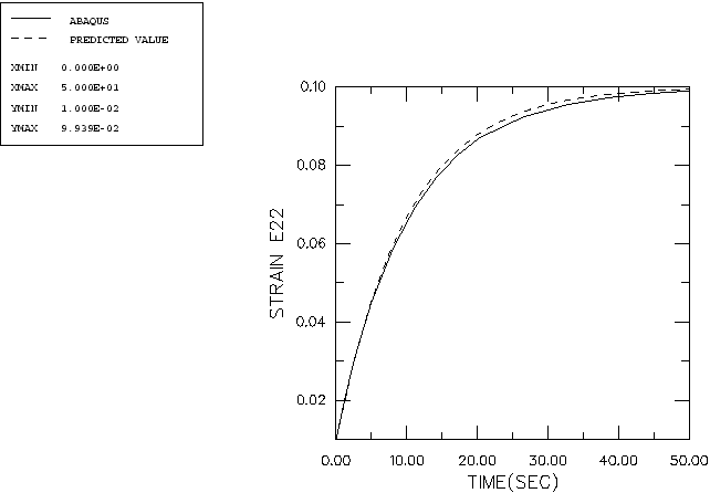
The solution obtained with the large-strain formulation differs negligibly from the small-strain solution. Abaqus automatically converts frequency domain data into a time domain Prony series representation. The analysis results using Prony parameters calibrated from tabulated frequency-dependent moduli data are in good agreement with the analyses using time domain data directly.
Small-strain input data for this problem.
Small-strain input data for time domain analysis using Prony parameters calibrated from tabulated frequency-dependent moduli data.
Large-strain input data for this problem.
Large-strain input data for this problem using Prony parameters calibrated from tabulated frequency-dependent moduli data.
Model using the three-dimensional 8-node brick element, C3D8.
Model using the 4-node plane stress element, CPS4.
Model using the 2-node truss element, T3D2.
*POST OUTPUT job for the restart file generated in viscorod_largestrain.inp.