Products: Abaqus/Standard Abaqus/Explicit
This example, taken from Collingwood et al. (1985), is intended to demonstrate the use of the time domain linear viscoelastic material model in conjunction with a temperature-time shift function. The model is a viscoelastic slab under plane strain restrained in all directions in its plane. We investigate the response of the slab after the temperature of its faces is raised suddenly to 100°.
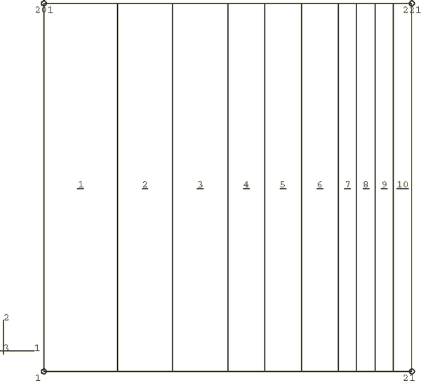
The slab has unit half-thickness. Since the problem is one-dimensional, the slab is modeled with a single row of plane strain continuum elements. In Abaqus/Standard a sequential thermal-stress analysis is performed with two-dimensional, 8-node heat transfer elements, DC2D8, used for the heat transfer analysis and the corresponding 8-node plane strain continuum elements, CPE8R, used for the stress analysis. The mesh is shown in Figure 3.1.21. In Abaqus/Explicit a coupled thermal-stress analysis is performed using first-order plane strain elements (CPE3T and CPE4RT) to model the slab. Twenty elements are used along the length of the slab in the Abaqus/Explicit simulation.
The initial temperature throughout the slab is 0°. The outside face of the slab, at ![]() 1, is instantaneously raised to 100°. The mesh (Figure 3.1.21) is finer toward
1, is instantaneously raised to 100°. The mesh (Figure 3.1.21) is finer toward ![]() 1, where the temperature gradient is expected to be highest. The resulting transient temperature distribution is written to the results file and used as input to the subsequent stress analysis. Plane strain is imposed in the Y-direction by setting
1, where the temperature gradient is expected to be highest. The resulting transient temperature distribution is written to the results file and used as input to the subsequent stress analysis. Plane strain is imposed in the Y-direction by setting ![]() 0 on the two faces of the mesh at
0 on the two faces of the mesh at ![]() 0 and
0 and ![]() 1. Symmetry about
1. Symmetry about ![]() 0 is also imposed.
0 is also imposed.
The thermal material properties are arbitrarily defined (in consistent units) as thermal conductivity (k) of 1.0, specific heat (c) of 1.0, and density (![]() ) of 1.0.
) of 1.0.
The viscoelastic material models (small-strain and large-strain) are the same as the ones used in “Viscoelastic rod subjected to constant axial load,” Section 3.1.1, with the addition of a temperature-time shift, defined with the *TRS option. The *TRS option uses the Williams-Landel-Ferry approximation,
![]()
The transient heat transfer problem is analyzed in Abaqus/Standard using the *HEAT TRANSFER procedure for a time period of 6 seconds, so the structure is allowed to come to thermal equilibrium. The integration procedure used in Abaqus/Standard for transient heat transfer analysis introduces a relationship between the minimum usable time increment and the element size and material properties. The guideline given in the User's Manual is
![]()
Automatic time incrementation is chosen by setting DELTMX on the *HEAT TRANSFER option to 20°. DELTMX controls the time incrementation by limiting the temperature change allowed at any point during an increment. Smaller values of DELTMX cannot be used in this problem because they result in time increments that are smaller than the minimum usable time increment described above. As a consequence, the thermal analysis is rather approximate. A finer mesh would be necessary to obtain more accurate results.
The stress analysis uses the temperature distribution obtained in the heat transfer analysis to define the thermal loading. The *VISCO procedure (“Quasi-static analysis,” Section 6.2.5 of the Abaqus Analysis User's Manual) is used with automatic incrementation, chosen by specifying a value for CETOL. CETOL is set to 2.0 × 10³, which is of the same order of magnitude as the maximum elastic strain. The time period is 6 seconds, and the initial suggested time increment is 5.0 × 10⁴ seconds to capture the high temperature gradients that occur very early in the analysis.
In Abaqus/Explicit the thermal and mechanical responses of the slab are determined simultaneously. The automatic time incrementation scheme available in Abaqus/Explicit is used to ensure numerical stability and to advance the solution in time.
The temperature distribution in the first part of the problem is given in Carslaw and Yeager (1959). Table 3.1.21 compares that exact solution with the Abaqus results after an elapsed time of one second.
Table 3.1.21 Exact solution compared to Abaqus results.
| Temperature | |||
|---|---|---|---|
| Carslaw and Yeager (1959) | Abaqus/Standard | Abaqus/Explicit | |
| 0.9 | 98.2 | 97.8 | 98.3 |
| 0.7 | 95.0 | 93.5 | 95.1 |
| 0.5 | 92.2 | 89.9 | 92.3 |
| 0.2 | 89.5 | 86.4 | 89.7 |
| 0.0 | 89.2 | 85.7 | 89.1 |
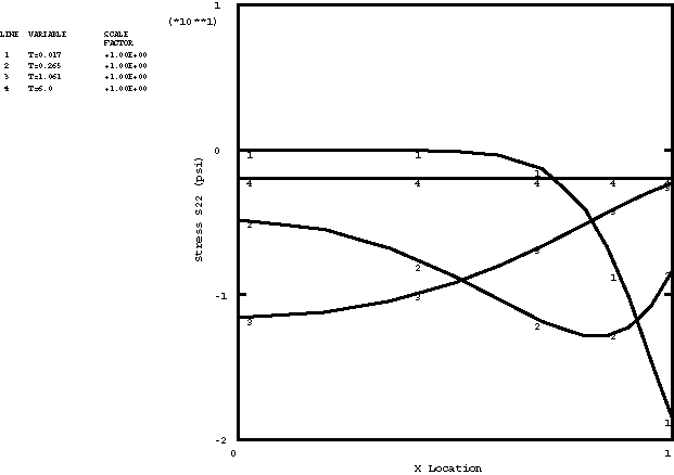
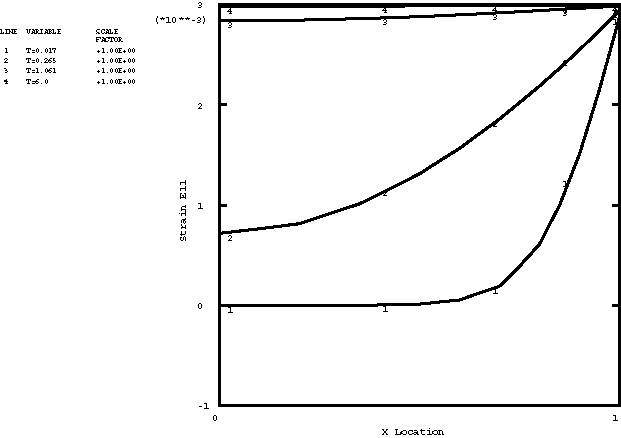
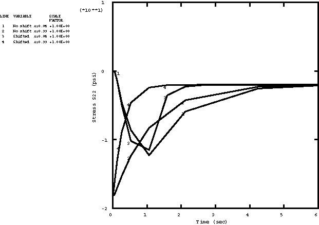
The stress and strain distributions at various times during the solution are shown in Figure 3.1.22 and Figure 3.1.23. The final stress in the slab is calculated as 0.0138 MPa (2 psi), while the final strain is 2.99 × 10³. Figure 3.1.24 shows the time history of the stress at the leftmost and rightmost integration points in the structure. Time histories for the same problem, solved without the temperature-time shift, are also shown in this figure. As expected, the shift considerably shortens the time required for the structure to reach equilibrium.
The equilibrium stress and strain distributions obtained from the stress analyses of the viscoelastic slab can be compared with those of an elastic slab whose properties correspond to the long-term properties of the viscoelastic material. The extensional relaxation function for the viscoelastic material is
![]()
By symmetry ![]() , and by the assumptions of plane strain
, and by the assumptions of plane strain ![]() 0. The slab is unrestrained in the X-direction, so
0. The slab is unrestrained in the X-direction, so ![]() 0. These conditions result in stress and strain distributions that follow the temperature distribution,
0. These conditions result in stress and strain distributions that follow the temperature distribution,
![]()
![]()
Heat transfer analysis.
Small-strain analysis of the viscoelastic slab with the temperature-time shift included.
Equivalent large-strain analysis.
User subroutine UTRS used in conjunction with viscoslabthermload_usr_utrs.inp.
Small-strain analysis of the viscoelastic slab with the temperature-time shift included; CPE3T elements.
Small-strain analysis of the viscoelastic slab with the temperature-time shift included; CPE4RT elements.
User subroutine VUTRS used in conjunction with viscoslabthermload_usr_cpe4rt.inp.
Large-strain analysis of the viscoelastic slab with the temperature-time shift included; CPE3T elements.
Large-strain analysis of the viscoelastic slab with the temperature-time shift included; CPE4RT elements.
To run the stress analyses without the shift, simply remove the *TRS option and the one data line that follows it from viscoslabthermload_smallstrain.inp, viscoslabthermload_largestrain.inp, viscoslabthermload_x_cpe3t.inp, viscoslabthermload_x_cpe4rt.inp, viscoslabthermload_xh_cpe3t.inp, and viscoslabthermload_xh_cpe4rt.inp.
Carslaw, H. S., and J. C. Yeager, Conduction of Heat in Solids, Clarendon Press, Oxford, 1959.
Collingwood, G. A., E. B. Becker, and T. Miller, User's Manual for the TEXVISC Computer Program, Morton Thiokol, Inc., Document Numbers U-85-4550A and U-85-4550B, 1985.