Products: Abaqus/Standard Abaqus/Explicit
Crack propagation analysis:
allows for five types of fracture criteria in Abaqus/Standard—critical stress at a certain distance ahead of the crack tip, critical crack opening displacement, crack length versus time, VCCT (the Virtual Crack Closure Technique), and the low-cycle fatigue criterion based on the Paris law;
allows for the VCCT fracture criterion in Abaqus/Explicit;
in Abaqus/Standard models quasi-static crack growth in two dimensions (planar and axisymmetric) for all types of fracture criteria and in three dimensions (solid, shells, and continuum shells) for VCCT and the low-cycle fatigue criteria; and
in Abaqus/Explicit models crack growth in three dimensions (solid, shells, and continuum shells) for VCCT criterion; and
requires that you define two distinct initially bonded contact surfaces between which the crack will propagate.
Potential crack surfaces are modeled as slave and master contact surfaces (see “Defining contact pairs in Abaqus/Standard,” Section 34.3.1). Any contact formulation except the finite-sliding, surface-to-surface formulation can be used. The predetermined crack surfaces are assumed to be initially partially bonded so that the crack tips can be identified explicitly by Abaqus/Standard. Initially bonded crack surfaces cannot be used with self-contact.
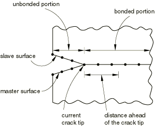
Define an initial condition to identify which part of the crack is initially bonded. You specify the slave surface, the master surface, and a node set that identifies the initially bonded part of the slave surface. The unbonded portion of the slave surface will behave as a regular contact surface. Either the slave surface or the master surface must be specified; if only the master surface is given, all of the slave surfaces associated with this master surface that have nodes in the node set will be bonded at these nodes.
If a node set is not specified, the initial contact conditions will apply to the entire contact pair; in this case, no crack tips can be identified, and the bonded surfaces cannot separate.
If a node set is specified, the initial conditions apply only to the slave nodes in the node set. Abaqus/Standard checks to ensure that the node set defined includes only slave nodes belonging to the contact pair specified.
By default, the nodes in the node set are considered to be initially bonded in all directions.
| Input File Usage: | *INITIAL CONDITIONS, TYPE=CONTACT |
For fracture criteria based on the critical stress, critical crack opening displacement, or crack length versus time, it is possible to bond the nodes in the node set (or the contact pair if a node set is not defined) only in the normal direction. In this case the nodes are allowed to move freely tangential to the contact surfaces. Friction (“Frictional behavior,” Section 35.1.5) cannot be specified if the nodes are bonded only in the normal direction.
Bonding only in the normal direction is typically used to model bonded contact conditions in Mode I crack problems where the shear stress ahead of the crack along the crack plane is zero.
| Input File Usage: | *INITIAL CONDITIONS, TYPE=CONTACT, NORMAL |
The crack propagation capability must be activated within the step definition to specify that crack propagation may occur between the two surfaces that are initially partially bonded. You specify the surfaces along which the crack propagates.
If the crack propagation capability is not activated for partially bonded surfaces, the surfaces will not separate; in this case the specified initial contact conditions would have the same effect as that provided by the tied contact capability, which generates a permanent bond between two surfaces during the entire analysis (see “Defining tied contact in Abaqus/Standard,” Section 34.3.7).
| Input File Usage: | *DEBOND, SLAVE=slave_surface_name, MASTER=master_surface_name |
Cracks can propagate from either a single crack tip or multiple crack tips. The crack propagation capability in Abaqus/Standard requires that the surfaces be initially partially bonded so that the crack tips can be identified. A contact pair can have crack propagation from multiple crack tips. However, only one crack propagation criterion is allowed for a given contact pair. Crack propagation along several contact pairs can be modeled by specifying multiple crack propagation definitions.
In Abaqus/Explicit potential crack surfaces are modeled as bonded general contact surfaces (see “Defining general contact interactions in Abaqus/Explicit,” Section 34.4.1) in the context of surface-based cohesive behavior (see “Surface-based cohesive behavior,” Section 35.1.10). Hence, the capability is available in three-dimensional analyses only and is implemented using a pure master-slave formulation. As is the case in Abaqus/Standard, the predetermined crack surfaces are assumed to be initially partially bonded so that the crack tips can be identified explicitly.
To identify which pair of surfaces determine the crack and which part of the crack is initially bonded, you must define and assign a contact clearance (see “Controlling initial contact status for general contact in Abaqus/Explicit,” Section 34.4.4). You first define a contact clearance to specify the node set that is initially bonded, and then you assign this contact clearance to a pair of two single-sided surfaces that define the crack. The unbonded portion behaves as a regular contact surface. The nodes in the node set are considered to be initially bonded in all directions.
The crack tip is identified only from the specified two surfaces and the node set. No attempt is made to determine a crack tip from all surfaces included in the general contact domain. Consequently, to be able to identify the crack tip, the surface including the specified node set must extend past the node set. Otherwise, the surfaces will not debond, and the crack cannot propagate.
You complete the definition of the crack propagation capability by defining a fracture-based cohesive behavior surface interaction. You activate the crack propagation by assigning it to the pair of surfaces that are initially partially bonded. If the fracture criterion is met, crack propagation occurs between these two surfaces. Cohesive behavior is also used to specify the elastic behavior of the bonds (see “Surface-based cohesive behavior,” Section 35.1.10).
If a fracture-based surface interaction is not assigned to a pair of surfaces, the crack definition is incomplete. Unlike Abaqus/Standard where the identified nodes will stay bonded if the crack is not activated, in Abaqus/Explicit the nodes identified by the contact clearance definition will separate without generating any interface stress.
Similar to Abaqus/Standard, cracks can propagate from single or multiple crack tips for the same pair of surfaces.
| Input File Usage: | Use the following options: |
*CONTACT CLEARANCE, NAME=clearance_name, SEARCH NSET=bonded_nset_name ** *SURFACE INTERACTION, NAME=interaction_name *COHESIVE BEHAVIOR *FRACTURE CRITERION ..** *CONTACT *CONTACT CLEARANCE ASSIGNMENT slave_surface, master_surface, clearance_name *CONTACT PROPERTY ASSIGNMENT slave_surface, master_surface, interaction_name |
You can specify the crack propagation criteria, as discussed below. Table 11.4.31 shows which criteria are supported by Abaqus/Standard and Abaqus/Explicit. Only one crack propagation criterion is allowed per contact pair even if multiple cracks are present.
| Crack propagation criterion | Abaqus/Standard | Abaqus/Explicit |
|---|---|---|
| Critical stress | Yes | No |
| Critical crack opening displacement | Yes | No |
| Crack length versus time | Yes | No |
| VCCT | Yes | Yes |
| Low-cycle fatigue | Yes | No |
Crack propagation analysis is carried out on a nodal basis. The crack-tip node debonds when the fracture criterion, f, reaches the value 1.0 within a given tolerance:
![]()
| Input File Usage: | *FRACTURE CRITERION, TOLERANCE= |
This criterion is available only in Abaqus/Standard.
If you specify a critical stress criterion at a critical distance ahead of the crack tip, the crack-tip node debonds when the local stress across the interface at a specified distance ahead of the crack tip reaches a critical value.
This criterion is typically used for crack propagation in brittle materials. The critical stress criterion is defined as
If the value of ![]() is not given or is specified as zero, it will be taken to be a very large number so that the shear stress has no effect on the fracture criterion.
is not given or is specified as zero, it will be taken to be a very large number so that the shear stress has no effect on the fracture criterion.
The distance ahead of the crack tip is measured along the slave surface, as shown in Figure 11.4.31. The stresses at the specified distance ahead of the crack tip are obtained by interpolating the values at the adjacent nodes. The interpolation depends on whether first-order or second-order elements are used to define the slave surface.
| Input File Usage: | *FRACTURE CRITERION, TYPE=CRITICAL STRESS, DISTANCE=n |
This criterion is available only in Abaqus/Standard.
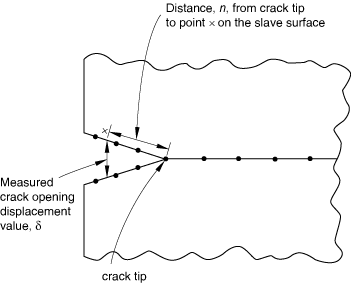
If you base the crack propagation analysis on the crack opening displacement criterion, the crack-tip node debonds when the crack opening displacement at a specified distance behind the crack tip reaches a critical value. This criterion is typically used for crack propagation in ductile materials.
The crack opening displacement criterion is defined as
![]()
You must supply the crack opening displacement versus cumulative crack length data. In Abaqus/Standard the cumulative crack length is defined as the distance between the initial crack tip and the current crack tip measured along the slave surface in the current configuration. The crack opening displacement is defined as the normal distance separating the two faces of the crack at the given distance.
You specify the position, n, behind the crack tip where the critical crack opening displacement is calculated. The value of this position must be specified as the length of the straight line joining the current crack tip and points on the slave and master surfaces (Figure 11.4.32).
Abaqus/Standard computes the crack opening displacement at that point by interpolating the values at the adjacent nodes. The interpolation depends on whether first-order or second-order elements are used to define the slave surface. An error message will be issued if the value of n is not within the end points of the contact pair.
| Input File Usage: | *FRACTURE CRITERION, TYPE=COD, DISTANCE=n |
In problems where the debonding surfaces lie on a symmetry plane, you can specify that Abaqus/Standard should consider only half of the user-specified crack opening displacement values. In this case the initial bonding must be in the normal direction only (see “Bonding only in the normal direction” above).
| Input File Usage: | *FRACTURE CRITERION, TYPE=COD, DISTANCE=n, SYMMETRY |
This criterion is available only in Abaqus/Standard.
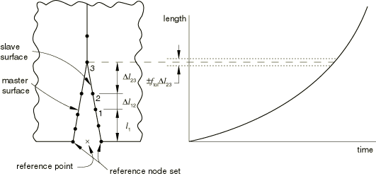
To specify the crack propagation explicitly as a function of total time, you must provide a crack length versus time relationship and a reference point from which the crack length is measured. This reference point is defined by specifying a node set. Abaqus/Standard finds the average of the current positions of the nodes in the set to define the reference point. During crack propagation the crack length is measured from this user-specified reference point along the slave surface in the deformed configuration. The time specified must be total time, not step time.
The fracture criterion, f, is stated in terms of the user-specified crack length and the length of the current crack tip. The length of the current crack tip from the reference point is measured as the sum of the straight line distance of the initial crack tip from the reference point and the distance between the initial crack tip and the current crack tip measured along the slave surface.
Referring to Figure 11.4.33, let node 1 be the initial location of the crack tip and node 3 be the current location of the crack tip. The distance of the current crack tip located at node 3 is given by
![]()
![]()
If geometric nonlinearity is considered in the step (“Procedures: overview,” Section 6.1.1), the reference point may move as the body deforms; you must ensure that this movement does not invalidate the crack length versus time criterion.
Abaqus/Standard does not extrapolate beyond the end points of your crack data. Therefore, if the first crack length specified is greater than the distance from the crack reference point to the first bonded node, the first bonded node will never debond and the crack will not propagate. In this case Abaqus/Standard will print warning messages in the message (.msg) file.
| Input File Usage: | *FRACTURE CRITERION, TYPE=CRACK LENGTH, NSET=name |
This criterion is available in both Abaqus/Standard and Abaqus/Explicit.
The Virtual Crack Closure Technique (VCCT) criterion uses the principles of linear elastic fracture mechanics (LEFM) and, therefore, is appropriate for problems in which brittle crack propagation occurs along predefined surfaces.
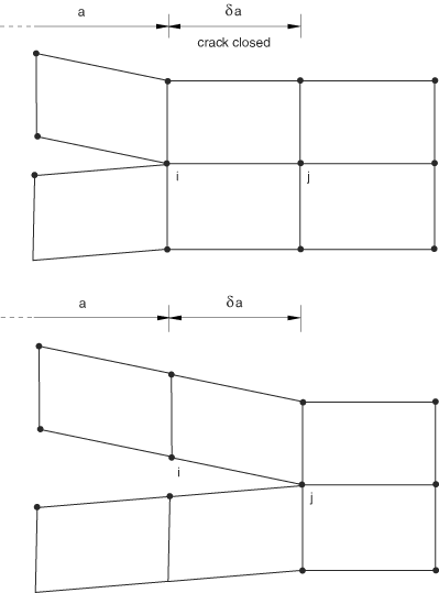
VCCT is based on the assumption that the strain energy released when a crack is extended by a certain amount is the same as the energy required to close the crack by the same amount. For example, Figure 11.4.34 illustrates the similarity between crack extension from i to j and crack closure at j.
Figure 11.4.34 Mode I: The energy released when a crack is extended by a certain amount is the same as the energy required to close the crack.
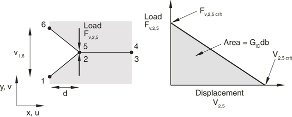
In Figure 11.4.35 nodes 2 and 5 will start to release when
![]()
In the general case involving Mode I, II, and III the fracture criterion is defined as
![]()
Abaqus provides three common mode-mix formulae for computing ![]() : the BK law, the power law, and the Reeder law models. The choice of model is not always clear in any given analysis; an appropriate model is best selected empirically.
: the BK law, the power law, and the Reeder law models. The choice of model is not always clear in any given analysis; an appropriate model is best selected empirically.
The BK law model is described in Benzeggagh (1996) by the following formula:
![]()
To define this model, you must provide ![]() and
and ![]() . This model provides a power law relationship combining energy release rates in Mode I, Mode II, and Mode III into a single scalar fracture criterion.
. This model provides a power law relationship combining energy release rates in Mode I, Mode II, and Mode III into a single scalar fracture criterion.
| Input File Usage: | *FRACTURE CRITERION, TYPE=VCCT, MIXED MODE BEHAVIOR=BK |
The power law model is described in Wu (1965) by the following formula:
![]()
To define this model, you must provide ![]() and
and ![]() .
.
| Input File Usage: | *FRACTURE CRITERION, TYPE=VCCT, MIXED MODE BEHAVIOR=POWER |
The Reeder law model is described in Reeder (2002) by the following formula:
![]()
![]()
To define this model, you must provide ![]() and
and ![]() . The Reeder law is best applied when
. The Reeder law is best applied when ![]() . When
. When ![]() , the Reeder law reduces to the BK law. The Reeder law applies only to three-dimensional problems.
, the Reeder law reduces to the BK law. The Reeder law applies only to three-dimensional problems.
| Input File Usage: | *FRACTURE CRITERION, TYPE=VCCT, MIXED MODE BEHAVIOR=REEDER |
You can define a VCCT criterion with varying energy release rates by specifying the critical energy release rates at the nodes.
If you indicate that the nodal critical energy rates will be specified, any constant critical energy release rates you specify are ignored, and the critical energy release rates are interpolated from the nodes. The critical energy release rates must be defined at all nodes on the slave surface.
| Input File Usage: | Use both of the following options: |
*FRACTURE CRITERION, TYPE=VCCT, NODAL ENERGY RATE *NODAL ENERGY RATE |
This criterion is available only in Abaqus/Standard.
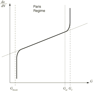
If you specify the low-cycle fatigue criterion, progressive delamination growth at the interfaces in laminated composites subjected to sub-critical cyclic loadings can be simulated. This criterion can be used only in a low-cycle fatigue analysis using the direct cyclic approach (“Low-cycle fatigue analysis using the direct cyclic approach,” Section 6.2.7). The onset and delamination growth are characterized by using the Paris law, which relates the relative fracture energy release rate to crack growth rates as illustrated in Figure 11.4.36. The fracture energy release rates at the crack tips in the interface elements are calculated based on the above mentioned VCCT technique.
The Paris regime is bounded by the energy release rate threshold, ![]() , below which there is no consideration of fatigue crack initiation or growth, and the energy release rate upper limit,
, below which there is no consideration of fatigue crack initiation or growth, and the energy release rate upper limit, ![]() , above which the fatigue crack will grow at an accelerated rate.
, above which the fatigue crack will grow at an accelerated rate. ![]() is the critical equivalent strain energy release rate calculated based on the user-specified mode-mix criterion and the bond strength of the interface. The formulae for calculating
is the critical equivalent strain energy release rate calculated based on the user-specified mode-mix criterion and the bond strength of the interface. The formulae for calculating ![]() have been provided above for different mixed mode fracture criteria. You can specify the ratio of
have been provided above for different mixed mode fracture criteria. You can specify the ratio of ![]() over
over ![]() and the ratio of
and the ratio of ![]() over
over ![]() . The default values are
. The default values are ![]() and
and ![]() .
.
| Input File Usage: | *FRACTURE CRITERION, TYPE=FATIGUE |
The onset of delamination growth refers to the beginning of fatigue crack growth at the crack tip along the interface. In a low-cycle fatigue analysis the onset of the fatigue crack growth criterion is characterized by ![]() , which is the relative fracture energy release rate when the structure is loaded between its maximum and minimum values. The fatigue crack growth initiation criterion is defined as
, which is the relative fracture energy release rate when the structure is loaded between its maximum and minimum values. The fatigue crack growth initiation criterion is defined as
![]()
Once the onset of delamination growth criterion is satisfied at the interface, the delamination growth rate, ![]() , can be calculated based on the relative fracture energy release rate,
, can be calculated based on the relative fracture energy release rate, ![]() . The rate of the delamination growth per cycle is given by the Paris law if
. The rate of the delamination growth per cycle is given by the Paris law if ![]()
![]()
At the end of cycle ![]() , Abaqus/Standard extends the crack length,
, Abaqus/Standard extends the crack length, ![]() , from the current cycle forward over an incremental number of cycles,
, from the current cycle forward over an incremental number of cycles, ![]() to
to ![]() by releasing at least one element at the interface. Given the material constants
by releasing at least one element at the interface. Given the material constants ![]() and
and ![]() , combined with the known node spacing
, combined with the known node spacing ![]() at the interface elements at the crack tips, the number of cycles necessary to fail each interface element at the crack tip can be calculated as
at the interface elements at the crack tips, the number of cycles necessary to fail each interface element at the crack tip can be calculated as ![]() , where j represents the node at the jthe crack tip. The analysis is set up to release at least one interface element after the loading cycle is stabilized. The element with the fewest cycles is identified to be released, and its
, where j represents the node at the jthe crack tip. The analysis is set up to release at least one interface element after the loading cycle is stabilized. The element with the fewest cycles is identified to be released, and its ![]() is represented as the number of cycles to grow the crack equal to its element length,
is represented as the number of cycles to grow the crack equal to its element length, ![]() . The most critical element is completely released with a zero constraint and a zero stiffness at the end of the stabilized cycle. As the interface element is released, the load is redistributed and a new relative fracture energy release rate must be calculated for the interface elements at the crack tips for the next cycle. This capability allows at least one interface element at the crack tips to be released after each stabilized cycle and precisely accounts for the number of cycles needed to cause fatigue crack growth over that length.
. The most critical element is completely released with a zero constraint and a zero stiffness at the end of the stabilized cycle. As the interface element is released, the load is redistributed and a new relative fracture energy release rate must be calculated for the interface elements at the crack tips for the next cycle. This capability allows at least one interface element at the crack tips to be released after each stabilized cycle and precisely accounts for the number of cycles needed to cause fatigue crack growth over that length.
If ![]() , the interface elements at the crack tips will be released by increasing the cycle number count,
, the interface elements at the crack tips will be released by increasing the cycle number count, ![]() , by one only.
, by one only.
After debonding, the traction between two surfaces is initially carried as equal and opposite forces at the slave node and the corresponding point on the master surface. The debonding force is released as the crack opens and advances. Once complete debonding has occurred at a point, the bond surfaces act like standard contact surfaces with associated interface characteristics. There are two different ways to release the debonding force, depending on the fracture criterion that you specify.
When you use the critical stress, critical crack opening displacement, or crack length versus time fracture criteria, you can define how this force is to be reduced to zero with time after debonding starts at a particular node on the bonded surface. You specify a relative amplitude, a, as a function of time after debonding starts at a node. Thus, suppose the force transmitted between the surfaces at slave node N is ![]() when that node starts to debond, which occurs at time
when that node starts to debond, which occurs at time ![]() . Then, for any time
. Then, for any time ![]() the force transmitted between the surfaces at node N is
the force transmitted between the surfaces at node N is ![]() . The relative amplitude must be 1.0 at the relative time 0.0 and must reduce to 0.0 at the last relative time point given.
. The relative amplitude must be 1.0 at the relative time 0.0 and must reduce to 0.0 at the last relative time point given.
The best choice of the amplitude curve depends on the material properties, specified loading, and the crack propagation criterion. If the stresses are removed too rapidly, the resulting large changes in the strains near the crack tip can cause convergence difficulties. For large-strain problems severe mesh distortion can also occur. For problems with rate-independent materials a linear amplitude curve is normally adequate. For problems with rate-dependent materials the stresses should be ramped off more slowly at the beginning of debonding to avoid convergence and mesh distortion difficulties. To reduce the likelihood of convergence and mesh distortion difficulties, you can reduce the value of the debond stress by 25% in 50% of the time to debond. The solution should not be strongly influenced by the details of the unloading procedure; if it is, this usually indicates that the mesh should be refined in the debond region.
| Input File Usage: | *DEBOND, SLAVE=slave, MASTER=master Data lines to define debonding amplitude curve |
For the VCCT criterion, when the energy release rate exceeds the critical value at a crack tip, you can either release the traction between the two surfaces at the crack tip immediately during the following increment or release the traction gradually during succeeding increments in such a way that the debonding force is brought to zero no later than the time at which the next node along the crack path begins to open. The latter approach is sometimes recommended to avoid sudden loss of stability when the crack tip is advanced.
Crack propagation analysis can be performed for static or dynamic overloadings using the following procedures:
It can also be performed for sub-critical cyclic fatigue loadings using the following procedure:When automatic incrementation is used for any criteria other than VCCT or low-cycle fatigue, you can specify the size of the time increment used just after debonding starts. By default, the time increment is equal to the last relative time specified. However, if a fracture criterion is met at the beginning of an increment, the size of the time increment used just after debonding starts will be set equal to the minimum time increment allowed in this step.
For fixed time incrementation the specified time increment value will be used as the time increment size after debonding starts if Abaqus/Standard finds it needs a smaller time increment than the fixed time increment size. The time increment size will be modified as required until debonding is complete.
| Input File Usage: | *DEBOND, SLAVE=slave, MASTER=master, TIME INCREMENT=t |
The simulation of structures with unstable propagating cracks is challenging and difficult. Nonconvergent behavior may occur from time to time. While the usual stabilization techniques (such as contact pair stabilization and static stabilization) can be used to overcome some convergence difficulties, localized damping is included for VCCT by using the viscous regularization technique. Viscous regularization damping causes the tangent stiffness matrix of the softening material to be positive for sufficiently small time increments.
| Input File Usage: | *FRACTURE CRITERION, TYPE=VCCT, VISCOSITY= |
For most crack propagation simulations using VCCT, the deformation can be nearly linear up to the point of the onset of crack growth; past this point the analysis becomes very nonlinear. In this case a linear scaling method can be used to effectively reduce the solution time to reach the onset of crack growth.
Suppose that an applied “trial” load at increment ![]() is just a fraction of the critical load at the onset time of crack growth,
is just a fraction of the critical load at the onset time of crack growth, ![]() . The following algorithm is used in Abaqus/Standard to quickly converge to the critical load state:
. The following algorithm is used in Abaqus/Standard to quickly converge to the critical load state:
| Input File Usage: | *CONTROLS, TYPE=VCCT LINEAR SCALING |
Crack propagation problems using the VCCT criterion are numerically challenging. The following tips will help you create a successful Abaqus/Standard model:
An analysis with the VCCT criterion requires small time increments. Abaqus/Standard tracks the location of the active crack front node by node when the VCCT criterion is used. Therefore, the crack front is allowed to advance only a single node forward in any single increment (although such an advance may take place across the entire crack front in three-dimensional problems). Because an analysis using the VCCT criterion provides detailed results of the growth of the crack, you will need small time increments, especially if the mesh is highly refined.
Three different types of damping can be used to aid convergence for a model using the VCCT criterion: contact stabilization, automatic or static stabilization, and viscous regularization. Contact and automatic stabilization are not specific to VCCT; they are built into Abaqus/Standard and are compatible with VCCT. Setting the value of the damping parameters is often an iterative procedure. If your VCCT model fails to converge due to unstable crack propagation, set the damping parameters to relatively high values and rerun the analysis. If the parameters are high enough, stable incrementation should return. However, the crack propagation behavior may have been modified by the damping forces and may not be physically correct. To monitor the energy absorbed by viscous damping, plot the damping energy and compare the results to the total strain energy in the model (ALLSE). When set properly, the value of the damping energy should be a small fraction of the total energy. Monitor the damping energy to ensure that the results of the VCCT simulation are reasonable in the presence of damping. When you use contact or automatic stabilization, Abaqus writes the damping energy to the variable ALLSD in the output database (.odb) file. When you use viscous regularization, Abaqus writes the damping energy to the variable ALLVD.
To maximize the accuracy of the debonding simulation, try to use matched meshes between the slave and master surfaces of the debonding contact pair.
If you do use a mismatched mesh, you can maximize the accuracy of the simulation by using the small-sliding, surface-to-surface formulation for the contact pair (see “Contact formulations in Abaqus/Standard,” Section 36.1.1).
Printing contact constraint information to the data (.dat) file allows you to review the status of the debonding contact pair at the beginning of the analysis. By printing detailed contact conditions to the message (.msg) file, you can track the incremental behavior of the advancing crack front during the analysis. For more information about these output requests, see “Output,” Section 4.1.1.
You can add a small clearance to the initially unbonded portion of the debonding contact pair (“Adjusting initial surface positions and specifying initial clearances in Abaqus/Standard contact pairs,” Section 34.3.5). The small clearance will help to eliminate unnecessary severe discontinuity iterations during incrementation as the crack begins to progress.
Do not use tie MPCs (“General multi-point constraints,” Section 33.2.2) for the slave surface in a debonding contact pair. Abaqus is unable to resolve the overconstraint presented by the MPC and the debonded contact state.
You must have continuous master debonding surfaces.
You may be able to help the analysis converge by adding geometric nonlinearity (even if small-sliding is used for the debonding contact pair). For more information, see “Geometric nonlinearity” in “General and linear perturbation procedures,” Section 6.1.2.
For two-dimensional models with contact pairs involving higher-order underlying elements, the initially unbonded portion must extend over complete element faces. In other words, the crack tip in a two-dimensional, higher-order model must start at a corner node on the quadratic slave surfaces. The crack tip must not start at a midside node.
Crack propagation problems using the VCCT criterion analyzed in Abaqus/Explicit benefit from the robustness of the general contact algorithm in the context of an explicit time integrator. Nevertheless, as is the case in Abaqus/Standard, these analyses remain challenging given the discontinuous nature of the fracture phenomenon. The following tips will help you create a successful Abaqus/Explicit model:
Dynamic effects are of utmost relevance when assessing the results from a debonding analysis using the VCCT criterion. In most cases experimental and/or theoretical data are available in quasi-static settings. You must ensure that the Abaqus/Explicit analysis generates low ratios of kinetic energy to internal energy (1% or less). In practical terms this requirement often translates into avoiding the use of mass scaling in the model. Use smooth amplitudes to drive the loading to help reduce the kinetic energy in the model. Running the analysis over a longer period of time will not help in most cases because bond breakage is an inherently fast and localized process.
If appropriate, use damping-like behavior in the materials associated with the debonding plates to reduce dynamic vibrations. Unlike Abaqus/Standard, where a pure static equilibrium is achieved at the end of a converged increment, in Abaqus/Explicit the bond breakage at a given location is associated with a dynamic overshoot beyond the static equilibrium position. If the vibrations are significant (kinetic energy is clearly observable), the dynamic overshoot at nodes behind the crack tip may lead to premature debonding of the crack tip.
To maximize the accuracy of the debonding simulation, use quad meshes between the slave and master surfaces of the debonding surfaces. Avoid using elements with aspect ratios greater than 2. In most cases mesh refinement will help with obtaining a realistic result.
Highly mismatched critical energy values between modes tend to induce crack propagation in continuously changing directions in a manner that may be unstable and unrealistic, particularly for modes II and III. Do not use such values unless experimental data suggest so.
Use frequent field output requests to evaluate the debonding evolution as the analysis progresses. In some cases this can point to nontrivial modeling deficiencies that are difficult to identify from a simple data check analysis.
Avoid the use of other constraints involving nodes on both surfaces of the debonding interface because the cohesive contact forces will compete with the constraint forces to achieve global equilibrium. Bond breakage might be hard to interpret in these cases.
Using VCCT to solve delamination problems is very similar to using cohesive elements in Abaqus. Table 11.4.32 describes the advantages and disadvantages of the two approaches.
For an example of the use of cohesive elements, see “Delamination analysis of laminated composites,” Section 2.7.1 of the Abaqus Benchmarks Manual. This example also shows the effect of viscous regularization on the predicted force-displacement response.
Table 11.4.32 Comparing VCCT and cohesive elements.
| VCCT | Cohesive Elements |
|---|---|
| Simulation (mechanics)-driven crack propagation along a known crack surface. | Simulation (mechanics)-driven crack propagation along a known crack surface. However, cohesive elements can also be placed between element faces as a mechanism for allowing individual elements to separate. |
| Models brittle fracture using LEFM only. | Model brittle or ductile fracture for LEFM or EPFM. Very general interaction modeling capability is possible. |
| Uses a surface-based framework. Does not require additional elements. | Require definition of the connectivity and interconnectivity of cohesive elements with the rest of the structure. For accuracy, the mesh of cohesive elements may need to be smaller than the surrounding structural mesh and the associated “cohesive zone.” As a result, cohesive elements may be more expensive. |
| Requires a pre-existing flaw at the beginning of the crack surface. Cannot model crack initiation from a surface that is not already cracked. | Can model crack initiation from initially uncracked surfaces. The crack initiates when the cohesive traction stress exceeds a critical value. |
| Crack propagates when strain energy release rate exceeds fracture toughness. | Crack propagates according to cohesive damage model, usually calibrated so that the energy released when the crack is fully open equals the critical strain energy release rate. |
| Multiple crack fronts/surfaces can be included. | Multiple crack fronts/surfaces can be included. |
| In Abaqus/Standard crack surfaces are rigidly bonded when uncracked. | Crack surfaces are joined elastically when uncracked in Abaqus/Standard. |
| Requires user-specified fracture toughness of the bond. | Require user-specified critical traction value and fracture toughness of the bond, as well as elasticity of the bonded surface. |
You must obtain the critical strain energy release properties of the bonded surfaces for VCCT. The procedure to obtain the critical strain energy release properties is beyond the scope of this manual; however, you can refer to the following ASTM test specifications for guidance:
ASTM D 5528-94a, “Standard Test Method for Mode I Interlaminar Fracture Toughness of Unidirectional Fiber-Reinforced Polymer Matrix Composites”
ASTM D 6671-01, “Standard Test Method for Mixed Mode I-Mode II Interlaminar Fracture Toughness of Unidirectional Fiber-Reinforced Polymer Matrix Composites”
ASTM D 6115-97, “Standard Test Method for Mode I Fatigue Delamination Growth Onset of Unidirectional Fiber-Reinforced Polymer Matrix Composites”
Initial contact conditions are used to identify which part of the slave surface is initially bonded, as explained earlier.
Boundary conditions should not be applied to any of the nodes on the master or slave crack surfaces, but they can be used to load the structure and cause crack propagation. Boundary conditions can be applied to any of the displacement degrees of freedom in a crack propagation analysis (“Boundary conditions in Abaqus/Standard and Abaqus/Explicit,” Section 32.3.1). In a low-cycle fatigue analysis, prescribed boundary conditions must have an amplitude definition that is cyclic over the step: the start value must be equal to the end value (see “Amplitude curves,” Section 32.1.2).
The following types of loading can be prescribed in a crack propagation analysis:
Concentrated nodal forces can be applied to the displacement degrees of freedom (1–6); see “Concentrated loads,” Section 32.4.2.
Distributed pressure forces or body forces can be applied; see “Distributed loads,” Section 32.4.3. The distributed load types available with particular elements are described in Part VI, “Elements.”
The following predefined fields can be specified in a crack propagation analysis, as described in “Predefined fields,” Section 32.6.1:
Although temperature is not a degree of freedom in stress/displacement elements, nodal temperatures can be specified as predefined fields. The specified temperature affects temperature-dependent critical stress and crack opening displacement failure criteria, if specified.
The values of user-defined field variables can be specified. These values affect field-variable-dependent critical stress and crack opening displacement failure criteria, if specified.
In a low-cycle fatigue analysis, the temperature values specified must be cyclic over the step: the start value must be equal to the end value (see “Amplitude curves,” Section 32.1.2). If the temperatures are read from the results file, you should specify initial temperature conditions equal to the temperature values at the end of the step (see “Initial conditions in Abaqus/Standard and Abaqus/Explicit,” Section 32.2.1). Alternatively, you can ramp the temperatures back to their initial condition values, as described in “Predefined fields,” Section 32.6.1.
Any of the mechanical constitutive models in Abaqus/Standard can be used to model the mechanical behavior of the cracking material. See Part V, “Materials.”
Regular, rectangular meshes give the best results in crack propagation analyses. Results with nonlinear materials are more sensitive to meshing than results with small-strain linear elasticity.
First-order elements generally work best for crack propagation analysis.
Line spring elements cannot be used in crack propagation analysis.
The VCCT and low-cycle fatigue criteria not only support two-dimensional models (planar and axisymmetric) but also three-dimensional models with contact pairs involving first-order underlying elements (solids, shells, and continuum shells). In Abaqus/Standard use of the VCCT criterion in two-dimensional models with contact pairs involving higher-order underlying elements is limited to crack fronts that are aligned with the corner nodes of the higher-order element faces. Use of the low-cycle fatigue criterion with contact pairs involving higher-order underlying elements is not supported.
Unless otherwise stated, the following discussions in this section are applied only to the critical stress, critical crack opening displacement, and crack length versus time criteria.
At the start of an analysis Abaqus/Standard will scan the partially bonded surfaces and identify all of the crack tips that are present in the model. The initial contact status of all of the slave surface nodes is printed in the data (.dat) file. At this stage Abaqus/Standard will explicitly identify all the crack tips and mark them as crack 1, crack 2, etc. The slave and master surfaces that are associated with these cracks are also identified.
The initial contact status of all of the slave surface nodes is also printed in the data (.dat) file for the VCCT and low-cycle fatigue criteria.
By default, crack propagation information will be printed to the data file during the analysis. For each crack that is identified Abaqus/Standard will print out the initial and current crack-tip node numbers, accumulated incremental crack length (distance from the initial crack tip to the current crack tip, measured along the slave surface), and the current value of the user-specified fracture criterion used. Crack propagation information cannot be printed to the data file in Abaqus/Explicit.
| Input File Usage: | *DEBOND, SLAVE=slave, MASTER=master |
For example, if the crack opening displacement criterion is used, the printed output during the analysis will appear as follows in the data file:
     CRACK TIP LOCATION AND ASSOCIATED QUANTITIES
CRACK  SLAVE   MASTER  INITIAL  CURRENT  CUMULATIVE  CRITICAL
NUMBER SURFACE SURFACE CRACKTIP CRACKTIP INCREMENTAL COD
                       NODE #   NODE #   LENGTH

In Abaqus/Standard you can choose to write the crack propagation information to the results (.fil) file.
| Input File Usage: | *DEBOND, SLAVE=slave, MASTER=master, OUTPUT=FILE |
In Abaqus/Standard you can write the crack propagation information to both the data and the results files.
| Input File Usage: | *DEBOND, SLAVE=slave, MASTER=master, OUTPUT=BOTH |
In Abaqus/Standard you can control the output frequency in increments. By default, the crack-tip location and associated quantities will be printed every increment. Specify an output frequency of 0 to suppress crack propagation output.
| Input File Usage: | *DEBOND, SLAVE=slave, MASTER=master, FREQUENCY=f |
The following bond failure quantities can be requested as surface output (see “Output to the data and results files,” Section 4.1.2; “Abaqus/Standard output variable identifiers,” Section 4.2.1; and “Abaqus/Explicit output variable identifiers,” Section 4.2.2) for all fracture criteria:
DBT | The time when bond failure occurred. For the VCCT and low-cycle fatigue criteria, this is the time when debonding initiates. |
DBSF | Fraction of stress at bond failure that still remains. |
DBS | All components of remaining stress in the failed bond. |
DBS1i | 1i component of stress in the failed bond that remains ( |
CSDMG | Overall value of the scalar damage variable. |
BDSTAT | Bond state. The bond state varies between 1.0 (fully bonded) and 0.0 (fully unbonded). |
OPENBC | Relative displacement behind crack when the fracture criterion is met. |
CRSTS | All components of critical stress at failure |
CRSTS1i | 1i component of critical stress at failure ( |
ENRRT | All components of strain energy release rate. |
ENRRT1i | 1i component of strain energy release rate ( |
EFENRRTR | Effective energy release rate ratio, |
Abaqus/CAE provides support for the visualization of time-history plots and X–Y plots of the variables that are written to the output database.
Contour integrals can be requested for two-dimensional crack propagation analyses performed using the critical stress, critical crack opening displacement, or crack length versus time fracture criteria. If the contours are chosen so that the crack tip passes through the contour, the contour value will go to zero (as it should). Therefore, in crack propagation analysis contour integrals should be requested far enough from the crack tip that the crack tip does not pass through the contour, which is easily done by including all nodes along the bond surface in the crack-tip node set specified. See “Contour integral evaluation,” Section 11.4.2, for details on contour integral output.
*HEADING
…
*BOUNDARY
Data lines to specify zero-valued boundary conditions
*INITIAL CONDITIONS, TYPE=CONTACT (, NORMAL)
Data lines to specify initial conditions
*SURFACE, NAME=slave
Data lines to define slave surface
*SURFACE, NAME=master
Data lines to define master surface
**
*CONTACT PAIR
slave, master
**
*STEP (, NLGEOM)
*STATIC or *VISCO or *COUPLED TEMPERATURE-DISPLACEMENT
*DEBOND, SLAVE=slave, MASTER=master
Data lines to define debonding amplitude curve
*FRACTURE CRITERION, TYPE=type, DISTANCE or NSET
Data lines to define fracture criterion
*BOUNDARY
Data lines to define zero-valued or nonzero boundary conditions
*CLOAD and/or *DLOAD and/or *TEMPERATURE and/or *FIELD
Data lines to define loading
**
*CONTOUR INTEGRAL, CONTOURS=n, TYPE=type
**Contour integrals can be requested in a two-dimensional crack propagation analysis
*CONTACT PRINT
DBT, DBSF, DBS
*EL PRINT
JK,
*END STEP
**
*STEP
*DIRECT CYCLIC, FATIGUE
*DEBOND, SLAVE=slave, MASTER=master
*FRACTURE CRITERION, TYPE=FATIGUE
Data lines to define material constants used in Paris law and  fracture criterion
*BOUNDARY
Data lines to define zero-valued or nonzero cyclic  boundary conditions
*CLOAD and/or *DLOAD and/or *TEMPERATURE and/or *FIELD
Data lines to define cyclic loading
**
*END STEP
**
*HEADING
…
*BOUNDARY
Data lines to specify zero-valued boundary conditions
*SURFACE, NAME=slave
Data lines to define slave surface
*SURFACE, NAME=master
Data lines to define master surface
**
*CONTACT CLEARANCE, NAME=clearance_name,
SEARCH NSET=initially_bonded_nodeset_name
*SURFACE INTERACTION, NAME=interaction_name
*COHESIVE BEHAVIOR
Data lines to specify elastic behavior
*FRACTURE CRITERION, TYPE=VCCT, MIXED MODE BEHAVIOR=BK
**
*STEP
*DYNAMIC, EXPLICIT
*CONTACT
*CONTACT CLEARANCE ASSIGNMENT
Data lines to assign a clearance name to a surface pair
*CONTACT PROPERTY ASSIGNMENT
Data lines to assign a surface interaction to a surface pair
*END STEP
**
Benzeggagh, M., and M. Kenane, “Measurement of Mixed-Mode Delamination Fracture Toughness of Unidirectional Glass/Epoxy Composites with Mixed-Mode Bending Apparatus,” Composite Science and Technology, vol. 56 439, 1996.
Reeder, J., S. Kyongchan, P. B. Chunchu, and D. R.. Ambur, “Postbuckling and Growth of Delaminations in Composite Plates Subjected to Axial Compression”43rd AIAA/ASME/ASCE/AHS/ASC Structures, Structural Dynamics, and Materials Conference, Denver, Colorado, vol. 1746, p. 10, 2002.
Wu, E. M., and R. C. Reuter Jr., “Crack Extension in Fiberglass Reinforced Plastics,” T and M Report, University of Illinois, vol. 275, 1965.