Product: Abaqus/CFD
Two-dimensional turbulent flow in a plane channel is used to verify the Spalart-Allmaras model. This canonical problem uses a simple geometry and permits direct comparison with the “law of the wall.”
Experimental evidence and dimensional analysis on flat-plate boundary layers and channel flows indicate that the hydrodynamically fully developed velocity profile collapses to a universal velocity profile when normalized with appropriated viscous units. This result is known as the law of the wall and is composed of three main regions in channel flows explained by Pope (2000).
The inner layer: In this region the viscous stress dominates and the mean velocity profile exhibits a linear profile.
The outer layer: In this region the turbulent stresses dominate and the mean velocity profile exhibits a logarithmic profile.
The buffer layer: In this region—a transition zone—both the viscous and turbulent stresses are important. The velocity profile exhibits a smooth transition that connects the linear and logarithmic regions.
The inner and outer profiles are described below. The nondimensional velocity, ![]() , and wall-normal distance,
, and wall-normal distance, ![]() , are defined as
, are defined as
![]()
![]()
![]()
![]()
![]()
The turbulent flow in a plane channel is characterized by a Reynolds number that uses the friction velocity and the channel half-width (H/2). The Reynolds number based on friction velocity is
![]()
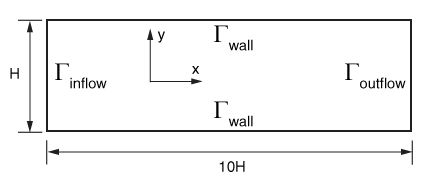
The model consists of a two-dimensional rectangular domain of dimension 10H in the x-direction, H in the y-direction, and 0.2H in the spanwise (out-of-plane) z-direction. Here, the channel height, H, is used to parameterize the domain geometry (see Figure 3.3.21).
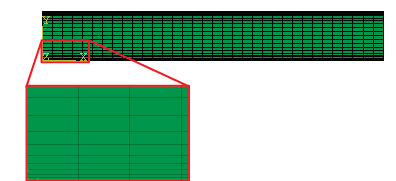
Mesh:
Due to the complexity of turbulent flows, the meshes need to be designed carefully to capture all the relevant turbulent scales of the problem and to satisfy the requirements of the turbulent model. For wall-bounded flows it is required that the wall-normal resolution (![]() ) reach the inner layer of the flow. Here, the near-wall resolution is defined as the location of the cell center of the first element cell adjacent to the wall. This constraint also applies to the Spalart-Allmaras model, which needs to resolve the inner layer requiring a near-wall resolution in the order of
) reach the inner layer of the flow. Here, the near-wall resolution is defined as the location of the cell center of the first element cell adjacent to the wall. This constraint also applies to the Spalart-Allmaras model, which needs to resolve the inner layer requiring a near-wall resolution in the order of ![]() to provide accurate predictions. Consequently, the meshes used in this study are designed keeping this restriction in mind. The finest mesh uses a near-wall resolution of
to provide accurate predictions. Consequently, the meshes used in this study are designed keeping this restriction in mind. The finest mesh uses a near-wall resolution of ![]() with a streamwise and spanwise resolution of
with a streamwise and spanwise resolution of ![]() and
and ![]() , respectively. The resolution in the streamwise direction could be relaxed more, but it was desired to maintain a relatively fine resolution to eliminate any dependence on the x-direction from the convergence study.
, respectively. The resolution in the streamwise direction could be relaxed more, but it was desired to maintain a relatively fine resolution to eliminate any dependence on the x-direction from the convergence study.
Five meshes, summarized in Table 3.3.21, were created.
Table 3.3.21 Mesh description.
| Mesh | Number of nodes ( | Number of elements | h/H | |
|---|---|---|---|---|
| 1 | 50, 23, 2 | 1078 | 1.013 × 10² | 4.00 |
| 2 | 50, 45, 2 | 2156 | 5.063 × 10³ | 2.00 |
| 3 | 50, 91, 2 | 4410 | 2.532 × 10³ | 1.00 |
| 4 | 50, 135, 2 | 6566 | 1.687 × 10³ | 0.66 |
| 5 | 50, 181, 2 | 8820 | 1.266 × 10³ | 0.50 |
![]()
![]()
![]()
![]()
The node distribution is accomplished in the following form. The nodes in the streamwise direction are uniformly distributed, while the nodes in the wall-normal direction from the walls to the middle of the channel are distributed using a hyperbolic-tangent distribution:
![]()
Boundary conditions:
The boundary conditions applied to the model are shown schematically in Figure 3.3.21. At the inflow surface, ![]() , the fluid pressure
, the fluid pressure ![]() is specified. At the top and bottom surfaces,
is specified. At the top and bottom surfaces, ![]() , the no-slip/no-penetration boundary conditions
, the no-slip/no-penetration boundary conditions ![]() are specified. For the turbulence model the Spalart-Allmaras turbulent viscosity
are specified. For the turbulence model the Spalart-Allmaras turbulent viscosity ![]() is set to zero, and the wall-normal distance is set to zero as well. At the outflow surface,
is set to zero, and the wall-normal distance is set to zero as well. At the outflow surface, ![]() , an outflow boundary condition (traction-free) is specified by setting the pressure
, an outflow boundary condition (traction-free) is specified by setting the pressure ![]() to zero. The normal gradients of velocities and Spalart-Allmaras viscosity,
to zero. The normal gradients of velocities and Spalart-Allmaras viscosity, ![]() , are automatically set to zero for this boundary. These conditions correspond to the well-known natural or “do-nothing” boundary condition. Finally, the two-dimensional nature of the problem is enforced by prescribing the out-of-plane velocity,
, are automatically set to zero for this boundary. These conditions correspond to the well-known natural or “do-nothing” boundary condition. Finally, the two-dimensional nature of the problem is enforced by prescribing the out-of-plane velocity, ![]() , to be zero everywhere on the domain surface and by using only one element through the thickness (along the spanwise direction).
, to be zero everywhere on the domain surface and by using only one element through the thickness (along the spanwise direction).
Initial conditions:
The initial velocity, V, is set to zero everywhere in the flow domain. The Spalart-Allmaras turbulent viscosity is initialized to five times the kinematic viscosity, ![]() .
.
Problem setup:
To set up the turbulent channel flow problem for the desired![]() , the following steps need to be conducted:
, the following steps need to be conducted:
Using the law of the wall estimate for the velocity at the center of the channel (![]() ), the friction velocity can be calculated:
), the friction velocity can be calculated:
![]()
The kinematic viscosity can be obtained from the Reynolds number since the friction velocity and channel height are available:
![]()
The mesh can be created for the specified near-wall resolution since all the information is available:
![]()
The inflow pressure is computed from the balance of mean x-momentum (see Pope, 2000):
![]()
![]()
After following Steps 1–4, the flow parameters obtained are ![]() =1 kg/m3,
=1 kg/m3, ![]() = 0.4783 × 101, and
= 0.4783 × 101, and ![]() =0.6190 × 10⁴. The total execution time was set to t = 1000 s to reach steady state in all meshes. The solver options are set to the defaults with the exception of the pressure Poisson equation (PPE) and momentum solver tolerance, which is set to 10 8 (default = 105).
=0.6190 × 10⁴. The total execution time was set to t = 1000 s to reach steady state in all meshes. The solver options are set to the defaults with the exception of the pressure Poisson equation (PPE) and momentum solver tolerance, which is set to 10 8 (default = 105).
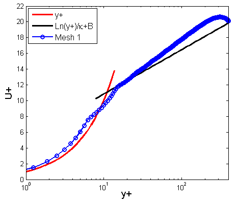
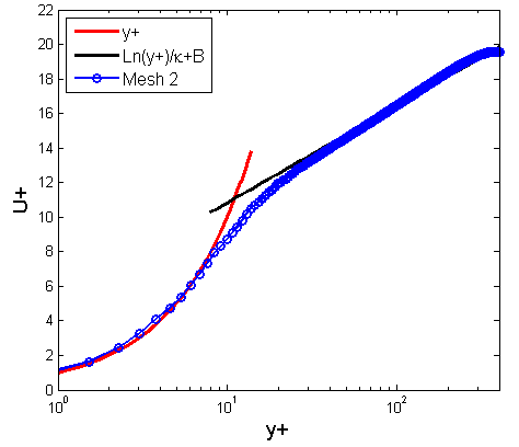
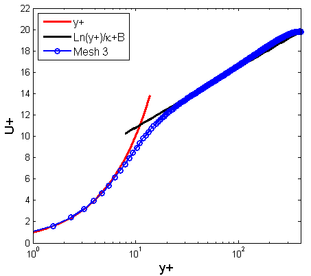
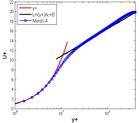
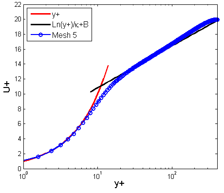
The mean velocity profiles normalized with wall units are presented for the five meshes in Figure 3.3.23 through Figure 3.3.27. The velocity profiles are shifted on the y-axis to improve the presentation of the results. For the present calculations the friction coefficient is computed directly from the mean velocity profile
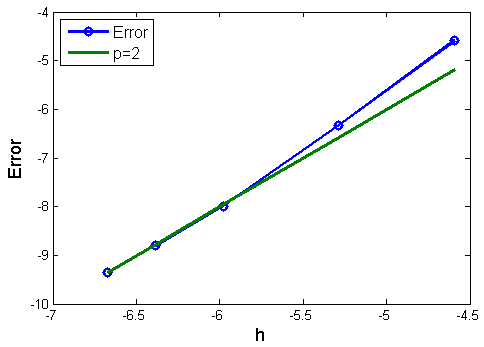
The rate of spatial convergence of the code can be estimated using the results computed on the five meshes. Following ASME V&V 20-2009, the error in the numerical solution can be computed as
![]()
To estimate the convergence rate, we use the computed friction velocity obtained from the law of the wall equation (Step 1 in the problem setup) as the exact value to estimate the error of the simulations. Following ASME V&V 20-2009, the observed convergence between the two calculations can be approximated as
The observed convergence rates computed using the above equation are presented in Table 3.3.23 and Figure 3.3.28. The observed convergence rates tend to a value of ![]() in excellent agreement with the theoretical accuracy of the code.
in excellent agreement with the theoretical accuracy of the code.
The steady incompressible turbulent flow in a planar channel was successfully computed using Abaqus/CFD. The mean velocity profiles were found to be in good agreement with the well-known law of the wall solution. Furthermore, the estimated convergence rate for the Abaqus/CFD friction velocity was measured and found to be in close agreement with the theoretical second-order spatial accuracy of the code.
Mesh 1: coarser mesh with 1078 elements.
Mesh 2: coarse mesh with 2156 elements.
Mesh 3: mesh with 4410 elements.
Mesh 4: fine mesh with 6566 elements.
Mesh 5: finer mesh with 8820 elements.